
All figures (14)
![Figure 8. Relaxation of the secondary voltages following the shutdown of the primary current associated with the bipole [A, B] = [5 14]. (a) Secondary voltage recorded at electrodes #2 to #9 (see position in Fig. 7). (b) Secondary voltage recorded at electrodes #9 to #15 (see position in Fig. 7). The secondary voltages exhibit some strong IP effects, which are associated with the presence of the coal (the same experiment performed without coal does not exhibit such polarization effect). The voltage at t5 = 13 s is used as a temporal reference for the secondary voltages at the different measurement times (i.e. we consider that the secondary voltages has fully relaxed at this time).](/figures/figure-8-relaxation-of-the-secondary-voltages-following-the-3keu72x5.png) Figure 8. Relaxation of the secondary voltages following the shutdown of the primary current associated with the bipole [A, B] = [5 14]. (a) Secondary voltage recorded at electrodes #2 to #9 (see position in Fig. 7). (b) Secondary voltage recorded at electrodes #9 to #15 (see position in Fig. 7). The secondary voltages exhibit some strong IP effects, which are associated with the presence of the coal (the same experiment performed without coal does not exhibit such polarization effect). The voltage at t5 = 13 s is used as a temporal reference for the secondary voltages at the different measurement times (i.e. we consider that the secondary voltages has fully relaxed at this time).
Figure 8. Relaxation of the secondary voltages following the shutdown of the primary current associated with the bipole [A, B] = [5 14]. (a) Secondary voltage recorded at electrodes #2 to #9 (see position in Fig. 7). (b) Secondary voltage recorded at electrodes #9 to #15 (see position in Fig. 7). The secondary voltages exhibit some strong IP effects, which are associated with the presence of the coal (the same experiment performed without coal does not exhibit such polarization effect). The voltage at t5 = 13 s is used as a temporal reference for the secondary voltages at the different measurement times (i.e. we consider that the secondary voltages has fully relaxed at this time).![Figure 7. Sketch of the sandbox. The tank is filled with water-saturated sand and contains a target composed of burning coal placed in the cylindrical area located at the central part of the sandbox. The dots denote the 52 stainless electrodes that are used for data acquisition. Two current injections are performed at the electrodes pairs [A, B] = [5, 14] (red) and [31, 40] (blue), respectively. The electrode #1 is used as the reference electrode (Ref) for the voltage electrodes recording the secondary voltage decay. The tank is discretized with 1000 elements.](/figures/figure-7-sketch-of-the-sandbox-the-tank-is-filled-with-water-2z2nv5oe.png) Figure 7. Sketch of the sandbox. The tank is filled with water-saturated sand and contains a target composed of burning coal placed in the cylindrical area located at the central part of the sandbox. The dots denote the 52 stainless electrodes that are used for data acquisition. Two current injections are performed at the electrodes pairs [A, B] = [5, 14] (red) and [31, 40] (blue), respectively. The electrode #1 is used as the reference electrode (Ref) for the voltage electrodes recording the secondary voltage decay. The tank is discretized with 1000 elements.
Figure 7. Sketch of the sandbox. The tank is filled with water-saturated sand and contains a target composed of burning coal placed in the cylindrical area located at the central part of the sandbox. The dots denote the 52 stainless electrodes that are used for data acquisition. Two current injections are performed at the electrodes pairs [A, B] = [5, 14] (red) and [31, 40] (blue), respectively. The electrode #1 is used as the reference electrode (Ref) for the voltage electrodes recording the secondary voltage decay. The tank is discretized with 1000 elements. Figure 9. Tomogram of the electrical conductivity field at the fourth iteration (RMS = 5.7, convergence criteria: variation of the objective function <0.001 between two successive iterations). The tomogram shows an area of high conductivity which is located exactly where the coal is burning. This is consistent with the fact that burning coal exhibits a strong conductivity.
 Figure 16. Inverted chargeability versus time in two arbitrary cells belonging to the computation domain. (a) Cell 1. (b) Cell 2. We chose these two arbitrary cells of the simulation domain in which we plot the intrinsic chargeability decay (blue dots) and its fitting with a time domain Cole–Cole relaxation model. By fitting the chargeability decay in each cell, we recover a value of M0, τand con the corresponding cell.
 Figure 15. Initial chargeability, relaxation time and Cole–Cole exponent fields. (a) Initial chargeability. (b) Relaxation time (c) Frequency exponent. We represent τ and c only in the region characterized by high values of M0 (>0.15). Indeed, the distribution of M0 shows high polarization effects where the coal is burning. The τ values are the highest (around 1.5 s) in the region where the coal is burning, while the values of c remain relatively high (greater than 0.9), suggesting that the polarization of the burning coal can be approximated with a Debye model.
![Figure 3. Geometry of the synthetic experiment. For this case, we used a 0.5m×0.5m×0.5m domain with insulating boundary conditions (simulating a sandbox experiment). In this domain, we place 24 electrodes denoted by the dots in the figure. These electrodes are placed in such a way that they encircle the central arc of the tank, where the polarizable body is placed. For the purpose of this experiment, 2 current injection/retrieval pair [A, B] have been performed at the bipoles [23, 28] and [7, 10], respectively. The electrode #1 is used as reference electrode for the secondary voltages. This box is discretized with 1000 elements.](/figures/figure-3-geometry-of-the-synthetic-experiment-for-this-case-17zgyhpc.png) Figure 3. Geometry of the synthetic experiment. For this case, we used a 0.5m×0.5m×0.5m domain with insulating boundary conditions (simulating a sandbox experiment). In this domain, we place 24 electrodes denoted by the dots in the figure. These electrodes are placed in such a way that they encircle the central arc of the tank, where the polarizable body is placed. For the purpose of this experiment, 2 current injection/retrieval pair [A, B] have been performed at the bipoles [23, 28] and [7, 10], respectively. The electrode #1 is used as reference electrode for the secondary voltages. This box is discretized with 1000 elements.
Figure 3. Geometry of the synthetic experiment. For this case, we used a 0.5m×0.5m×0.5m domain with insulating boundary conditions (simulating a sandbox experiment). In this domain, we place 24 electrodes denoted by the dots in the figure. These electrodes are placed in such a way that they encircle the central arc of the tank, where the polarizable body is placed. For the purpose of this experiment, 2 current injection/retrieval pair [A, B] have been performed at the bipoles [23, 28] and [7, 10], respectively. The electrode #1 is used as reference electrode for the secondary voltages. This box is discretized with 1000 elements.![Figure 11. Primary current density distributions. (a) Primary current distribution for the electrode bipole [A, B] = [31; 40]. (b) Primary current distribution for the electrode bipole [A, B] = [5 14]. The primary current distributions are very high in the vicinity of the sources, that is, around the current injection electrodes. We observe the presence pattern of sensitivity of the primary current density, and as we get far from this pattern, the sensitivity drops and the current density becomes very small.](/figures/figure-11-primary-current-density-distributions-a-primary-1xz384yi.png) Figure 11. Primary current density distributions. (a) Primary current distribution for the electrode bipole [A, B] = [31; 40]. (b) Primary current distribution for the electrode bipole [A, B] = [5 14]. The primary current distributions are very high in the vicinity of the sources, that is, around the current injection electrodes. We observe the presence pattern of sensitivity of the primary current density, and as we get far from this pattern, the sensitivity drops and the current density becomes very small.
Figure 11. Primary current density distributions. (a) Primary current distribution for the electrode bipole [A, B] = [31; 40]. (b) Primary current distribution for the electrode bipole [A, B] = [5 14]. The primary current distributions are very high in the vicinity of the sources, that is, around the current injection electrodes. We observe the presence pattern of sensitivity of the primary current density, and as we get far from this pattern, the sensitivity drops and the current density becomes very small. Figure 2. Step-by-step summary of the inversion methodology. ERT corresponds to electrical resistivity tomography. The first step is to determine the electrical conductivity field from which the kernel used to invert the secondary voltages is computed. For each injected current at a bipole (A, B), we compute the secondary source current density using a linear inversion procedure (second step). The chargeability is given as the ratio between the secondary and the primary current distribution. Finally the relaxation time and the Cole–Cole frequency exponent are determined at each cell by fitting the inverted data and a variety of strategies can be used for this final step (third step).
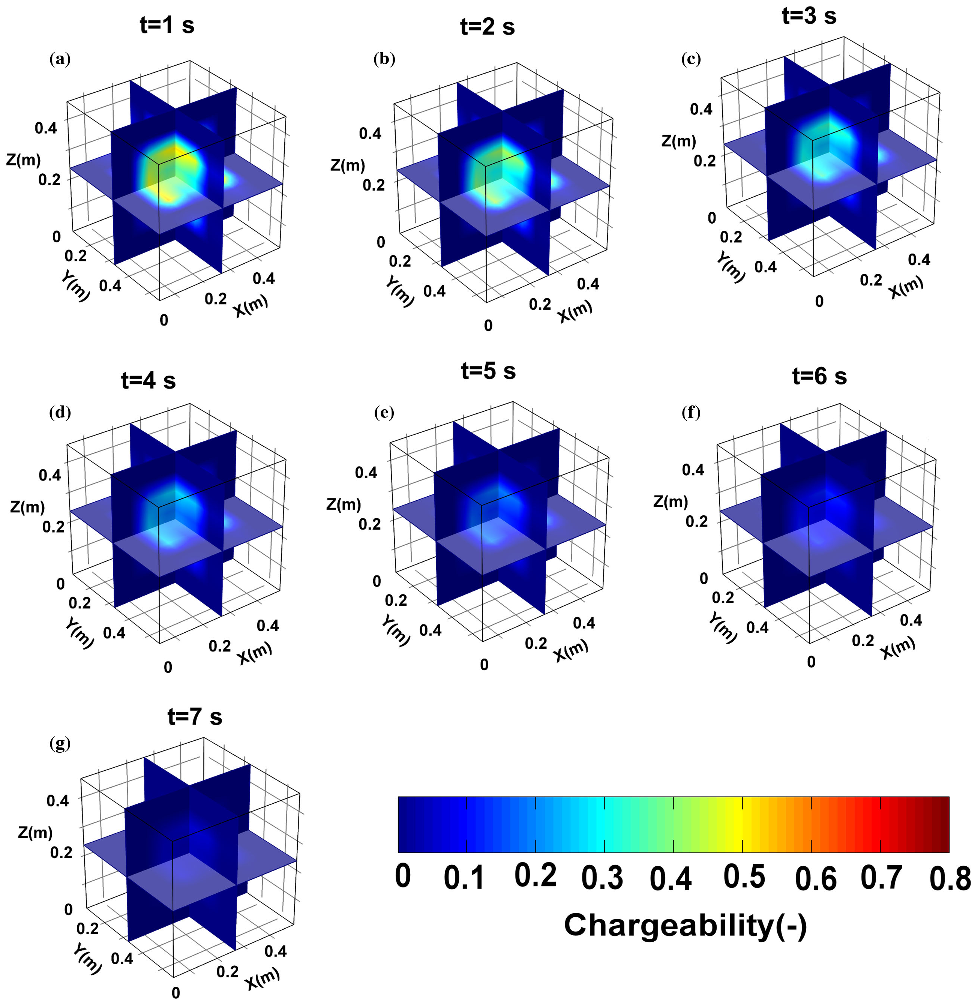 Figure 6. Intrinsic chargeability decay during each time window after the primary current was shut off. Note that the chargeability at time 0 is obtained jointly with the relaxation time and the frequency exponent using the curve fitting method. It cannot be inferred from the linear inversion because the potential is not recorded at time 0 since early times are contaminated with electromagnetic coupling effects.
 Figure 14. Intrinsic chargeability as a function of the elapsed time after the shutdown of the primary current. (a–h) We observe the intrinsic chargeability temporal evolution just after the primary current is shut down. The intrinsic chargeability exhibits a high anomaly in the central area of the tank, which is associated with the burning coal. The amplitude of the anomaly keeps decreasing over time, until it completely vanishes.
 Figure 1. Polarization of a porous material. (a) Recorded voltage at the two voltage electrodes M and N as a function of time. The primary current is applied for the period Ton (from –T to 0). The secondary voltage is measured after the primary current is shut down (during Toff). (b) Polarization of the grains. The instantaneous conductivity σ∞ is defined right after the application of the primary current. All the charge carriers are mobile. After a long time, the some of the charge carriers are blocked. This defined the direct current conductivity σ 0.
 Figure 12. Secondary current density distribution. This distribution is here estimated at t = 0.16 s. It shows an anomaly of high current density which indeed is located in the central area where the burning coal is located.
![Figure 13. Observed versus computed secondary voltages. (a) Comparison for bipole [A, B] = [31, 40]. (b) Comparison for bipole [A, B] = [5, 14]. We plot the true and estimated secondary voltages on all the electrodes at time t = 0.16 s. The computed voltages are obtained using the estimated source current density corresponding to the optimal solution of linear inverse problem.](/figures/figure-13-observed-versus-computed-secondary-voltages-a-1mfp1s1y.png) Figure 13. Observed versus computed secondary voltages. (a) Comparison for bipole [A, B] = [31, 40]. (b) Comparison for bipole [A, B] = [5, 14]. We plot the true and estimated secondary voltages on all the electrodes at time t = 0.16 s. The computed voltages are obtained using the estimated source current density corresponding to the optimal solution of linear inverse problem.
Figure 13. Observed versus computed secondary voltages. (a) Comparison for bipole [A, B] = [31, 40]. (b) Comparison for bipole [A, B] = [5, 14]. We plot the true and estimated secondary voltages on all the electrodes at time t = 0.16 s. The computed voltages are obtained using the estimated source current density corresponding to the optimal solution of linear inverse problem.![Figure 10. Observed versus computed resistances at the position of the 50 electrodes. (a) Observed versus computed resistances for bipole [A, B] = [31, 40]. (b) Observed versus computed resistances for bipole [A, B] = [5, 14]. The computed resistances reproduce the measured resistances. The latter were used as data for the electrical resistivity tomography.](/figures/figure-10-observed-versus-computed-resistances-at-the-26wp5wls.png) Figure 10. Observed versus computed resistances at the position of the 50 electrodes. (a) Observed versus computed resistances for bipole [A, B] = [31, 40]. (b) Observed versus computed resistances for bipole [A, B] = [5, 14]. The computed resistances reproduce the measured resistances. The latter were used as data for the electrical resistivity tomography.
Figure 10. Observed versus computed resistances at the position of the 50 electrodes. (a) Observed versus computed resistances for bipole [A, B] = [31, 40]. (b) Observed versus computed resistances for bipole [A, B] = [5, 14]. The computed resistances reproduce the measured resistances. The latter were used as data for the electrical resistivity tomography.
![Figure 8. Relaxation of the secondary voltages following the shutdown of the primary current associated with the bipole [A, B] = [5 14]. (a) Secondary voltage recorded at electrodes #2 to #9 (see position in Fig. 7). (b) Secondary voltage recorded at electrodes #9 to #15 (see position in Fig. 7). The secondary voltages exhibit some strong IP effects, which are associated with the presence of the coal (the same experiment performed without coal does not exhibit such polarization effect). The voltage at t5 = 13 s is used as a temporal reference for the secondary voltages at the different measurement times (i.e. we consider that the secondary voltages has fully relaxed at this time).](/figures/figure-8-relaxation-of-the-secondary-voltages-following-the-3keu72x5.webp)
![Figure 7. Sketch of the sandbox. The tank is filled with water-saturated sand and contains a target composed of burning coal placed in the cylindrical area located at the central part of the sandbox. The dots denote the 52 stainless electrodes that are used for data acquisition. Two current injections are performed at the electrodes pairs [A, B] = [5, 14] (red) and [31, 40] (blue), respectively. The electrode #1 is used as the reference electrode (Ref) for the voltage electrodes recording the secondary voltage decay. The tank is discretized with 1000 elements.](/figures/figure-7-sketch-of-the-sandbox-the-tank-is-filled-with-water-2z2nv5oe.webp)


![Figure 3. Geometry of the synthetic experiment. For this case, we used a 0.5m×0.5m×0.5m domain with insulating boundary conditions (simulating a sandbox experiment). In this domain, we place 24 electrodes denoted by the dots in the figure. These electrodes are placed in such a way that they encircle the central arc of the tank, where the polarizable body is placed. For the purpose of this experiment, 2 current injection/retrieval pair [A, B] have been performed at the bipoles [23, 28] and [7, 10], respectively. The electrode #1 is used as reference electrode for the secondary voltages. This box is discretized with 1000 elements.](/figures/figure-3-geometry-of-the-synthetic-experiment-for-this-case-17zgyhpc.webp)
![Figure 11. Primary current density distributions. (a) Primary current distribution for the electrode bipole [A, B] = [31; 40]. (b) Primary current distribution for the electrode bipole [A, B] = [5 14]. The primary current distributions are very high in the vicinity of the sources, that is, around the current injection electrodes. We observe the presence pattern of sensitivity of the primary current density, and as we get far from this pattern, the sensitivity drops and the current density becomes very small.](/figures/figure-11-primary-current-density-distributions-a-primary-1xz384yi.webp)


![Figure 13. Observed versus computed secondary voltages. (a) Comparison for bipole [A, B] = [31, 40]. (b) Comparison for bipole [A, B] = [5, 14]. We plot the true and estimated secondary voltages on all the electrodes at time t = 0.16 s. The computed voltages are obtained using the estimated source current density corresponding to the optimal solution of linear inverse problem.](/figures/figure-13-observed-versus-computed-secondary-voltages-a-1mfp1s1y.webp)
![Figure 10. Observed versus computed resistances at the position of the 50 electrodes. (a) Observed versus computed resistances for bipole [A, B] = [31, 40]. (b) Observed versus computed resistances for bipole [A, B] = [5, 14]. The computed resistances reproduce the measured resistances. The latter were used as data for the electrical resistivity tomography.](/figures/figure-10-observed-versus-computed-resistances-at-the-26wp5wls.webp)