
All figures (29)
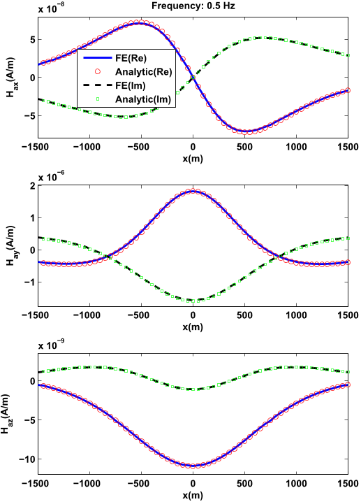 Fig. 5. A comparison between the finite element result and the 1D semi-analytical solution for the secondary magnetic field with a frequency of 0.5 Hz on the seafloor. The upper panel shows a comparison for the x component of secondary magnetic field at = −y 50 m; the middle panel shows a comparison for the y component of secondary magnetic field at y¼0; the lower panel shows a comparison for the z component of secondary magnetic field at = −y 50 m.
 Fig. 8. Plane view of the grid used for the model of the off-shore HC reservoir. The blue area indicates the reservoir and the red star represents the location of a dipole source. (For interpretation of the references to color in this figure caption, the reader is referred to the web version of this paper.)
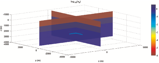 Fig. 6. 3D view of a model of the off-shore HC reservoir. The resistivity is shown in logarithmic scale.
 Fig. 7. Vertical section at y¼0 of the grid used for the model of the off-shore HC reservoir. The blue area indicates the reservoir and the red star represents the location of a dipole source. (For interpretation of the references to color in this figure caption, the reader is referred to the web version of this paper.)
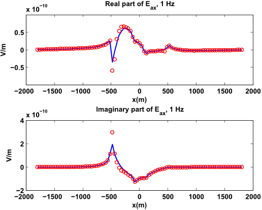 Fig. 28. Bathymetry model with the HC reservoir. A comparison of the x component of the anomalous electric field computed using the finite element (red circles) and integral equation (blue line) methods at y¼0 along the sea floor for a frequency of 1 Hz. (For interpretation of the references to color in this figure caption, the reader is referred to the web version of this paper.)
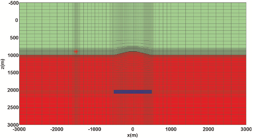 Fig. 27. X–Z section of the hexahedral grid for bathymetry model with a reservoir. The red star indicates the location of the dipole source oriented in the x direction. (For interpretation of the references to color in this figure caption, the reader is referred to the web version of this paper.)
 Fig. 26. Bathymetry model without HC reservoir. A comparison of the x component of the anomalous electric field computed using the finite element (red circles) and integral equation (blue line) methods at y¼0 along the sea floor for a frequency of 1 Hz. (For interpretation of the references to color in this figure caption, the reader is referred to the web version of this paper.)
 Fig. 24. A staircase approximation of the bathymetry model use in the framework of the integral equation method.
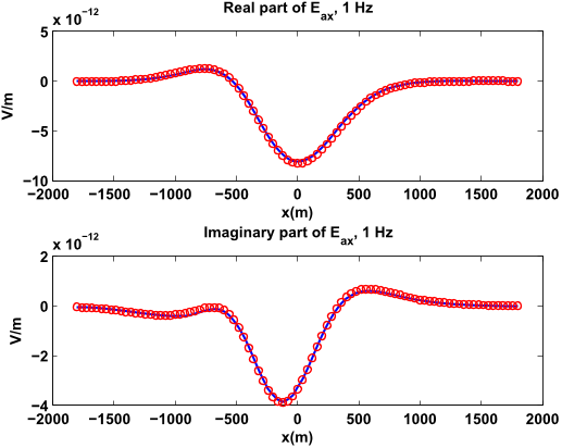 Fig. 25. Bathymetry model without HC reservoir. A comparison of the x component of the anomalous electric field computed using the finite element (red circles) and integral equation (blue line) methods at y¼0 and z¼500 m for a frequency of 1 Hz. (For interpretation of the references to color in this figure caption, the reader is referred to the web version of this paper.)
 Fig. 11. Model 1. A comparison of the x component of the background and total electric fields at y¼400 m for a frequency of 1 Hz. The solid blue line shows the background field while the dashed red line represents the total field. (For interpretation of the references to color in this figure caption, the reader is referred to the web version of this paper.)
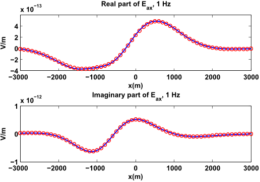 Fig. 10. Model 1. A comparison of the x component of the anomalous electric field computed using the finite element (red circles) and integral equation (blue line) methods at y¼0 for a frequency of 1 Hz. (For interpretation of the references to color in this figure caption, the reader is referred to the web version of this paper.)
 Fig. 9. Sparsity patterns of the FEM and FDM stiffness matrices for the 3D reservoir model. Panel (a) shows the sparsity pattern of edge-based finite element stiffness matrix (with 41,412,819 nozero entries), while panel (b) presents the sparsity of finite difference stiffness matrix (with 17,568,102 nozero entries) for the same model.
 Fig. 23. X–Z section of the hexahedral grid for bathymetry model without a reservoir. The red star indicates the location of the dipole source oriented in the x direction. (For interpretation of the references to color in this figure caption, the reader is referred to the web version of this paper.)
 Fig. 21. A comparison of normalized anomalous field at y¼0 for different 3D models for a frequency of 1 Hz.
 Fig. 22. A 3D view of a trapezoidal-type hill model of the seafloor bathymetry.
 Fig. 20. Model 4. A comparison of the x component of the background and total electric fields at y¼400 m for a frequency of 1 Hz. The solid blue line shows the background field while the dashed red line represents the total field. (For interpretation of the references to color in this figure caption, the reader is referred to the web version of this paper.)
 Fig. 1. An illustration of rectangular brick element. The number with circle indicates the node index and the number without circle is the index of edges.
 Fig. 14. Convergence plot of QMR solver for 3D reservoir Model 1 for the data with the frequency of 1 Hz compared to the convergence plots of the GMRES and BiCGSTAB solvers.
 Fig. 12. Model 1. A comparison of the x component of the anomalous electric field computed using the finite element (red circles) and integral equation (blue line) methods at y¼0 for a frequency of 0.1 Hz. (For interpretation of the references to color in this figure caption, the reader is referred to the web version of this paper.)
 Fig. 13. Model 1. A comparison of the x component of the anomalous electric field computed using the finite element (red circles) and integral equation (blue line) methods at y¼0 for a frequency of 0.5 Hz. (For interpretation of the references to color in this figure caption, the reader is referred to the web version of this paper.)
 Fig. 15. Model 2. A comparison of the x component of anomalous electric field computed using the finite element (red circles) and integral equation (blue line) methods at y¼0 for a frequency of 1 Hz. (For interpretation of the references to color in this figure caption, the reader is referred to the web version of this paper.)
 Fig. 2. (a) Hexahedral element in the xyz-coordinate system. (b) The same element transformed into a cubic element in the ξηζ-coordinate system.
 Fig. 29. Comparison of QMR convergence plots for different 3D reservoir models presented in this paper.
 Fig. 16. Model 2. A comparison of the x component of the background and total electric fields at y¼400 m for a frequency of 1 Hz. The solid blue line shows the background field while the dashed red line represents the total field. (For interpretation of the references to color in this figure caption, the reader is referred to the web version of this paper.)
 Fig. 19. Model 4. A comparison of the x component of anomalous electric field computed using the finite element (red circles) and integral equation (blue line) methods at y¼0 for a frequency of 1 Hz. (For interpretation of the references to color in this figure caption, the reader is referred to the web version of this paper.)
 Fig. 17. Model 3. A comparison of the x component of anomalous electric field computed using the finite element (red circles) and integral equation (blue line) methods at y¼0 for a frequency of 1 Hz. (For interpretation of the references to color in this figure caption, the reader is referred to the web version of this paper.)
 Fig. 18. Model 3. A comparison of the x component of the background and total electric fields at y¼400 m for a frequency of 1 Hz. The solid blue line shows the background field while the dashed red line represents the total field. (For interpretation of the references to color in this figure caption, the reader is referred to the web version of this paper.)
 Fig. 4. A comparison between finite element result and the 1D semi-analytical solution for the secondary electric field with a frequency of 0.5 Hz on the seafloor. The upper panel shows a comparison for the x component of secondary electric field at y¼0; the middle panel shows a comparison for the y component of secondary electric field at = −y 50 m; the lower panel shows a comparison for the z component of secondary electric field at y¼0.
 Fig. 3. Rectangular mesh for a horizontally layered geoelectrical model. The red resistive layer is embedded in sediments below seawater. The red star in this figure indicates the excitation dipole source. (For interpretation of the references to color in this figure caption, the reader is referred to the web version of this paper.)


