
All figures (14)
 Fig. 4. Temporal mean and standard deviation images of the 85-GHz vertically polarized SSM/I channel. These were generated using 44 descending single-pass images corresponding to days 245–264 of 1992. The left panel is the mean image, and the right panel is the standard deviation image. The boxes define two 2 2 subregions used later in the assessment of algorithm effectiveness. One is an example of a cloudy region, and the other is a region with little or no distortion. The band in the lower-right area of the standard deviation image results from atmospheric distortions affecting only some passes.
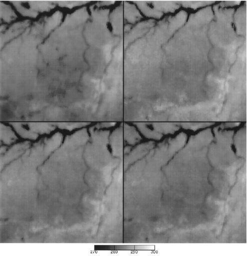 Fig. 6. SSM/I 37-V Brazil region composite images. From top left to bottom right: mean, second-highest value, MMA, and hybrid.
 TABLE I SSM/I CHANNELS
 Fig. 8. Cloudy region temporal and spatial measurement histograms for all SSM/I vertically polarized channels. A log vertical scale has been used to emphasize the tails of the distributions. These tails correspond to atmospheric distortions that lower the overall brightness temperature.
 Fig. 7. SSM/I 85-V Brazil region composite images. From top left to bottom right: mean, second-highest value, MMA, and hybrid.
 Fig. 9. Clear region temporal and spatial measurement histograms for all SSM/I vertically polarized channels. Compare these distributions with those in Fig. 10. The lack of tails on the distributions indicates the absence of significant atmospheric distortions.
 Fig. 1. Individual SSM/I swath examples of temporal atmospheric distortions. These images were created by assigning the closest measurement value to each pixel. Columns (from left to right) correspond to 1992 Julian Days 245, 248, 261, and 264 of the passes. Rows (from top to bottom) indicate SSM/I channels 19 V, 22 V, 27 V, and 85 V.
 Fig. 11. SSM/I 85-V clear region cloud-removal composite images. From top left to bottom right: mean, second-highest value, MMA, and hybrid.
 Fig. 12. SSM/I 85-GHz vertical channel cloudy region spatial brightness temperature distributions for each cloud-removal algorithm. The temporal and spatial measurement distribution has been plotted to provide a reference.
 Fig. 10. SSM/I 85-V cloudy region cloud-removal composite images. From top left to bottom right: mean, second-highest value, MMA, and hybrid.
 TABLE III PIXEL VALUE AVERAGES AND STANDARD DEVIATIONS OF EACH ALGORITHM COMPOSITE IMAGE FOR THE CLOUDY AND CLEAR REGIONS
 Fig. 2. Illustration of hypothetical radiometric measurement distribution for a cloudy region. (a) Sample discrete ensemble. (b) Variance of the modified maximum and second-highest value.
 Fig. 13. SSM/I 85-GHz vertical channel clear region spatial brightness temperature distributions for each cloud-removal algorithm. The temporal and spatial measurement distribution has been plotted to provide a reference.
 Fig. 3. Illustration of hypothetical radiometric measurement distribution for a clear region. (a) Sample discrete ensemble. (b) Variance of the modified maximum and second-highest value.


