
All figures (13)
 Figure 3. Time evolution of the SXR–evaluated W density profiles with ICRH (a-c) and ECRH (d-f) at high (time window from 2.2s to 3.0) (a,b) and low (time window from 6.6s to 7.5s) (c,d) RF power density, and (e,f) corresponding time averaged W density profiles (solid) compared to the corresponding time averaged electron density profiles (dashed). all normalized to their values at r/a = 0.4. In (e,f), full squares and full circles are the W corresponding density measurements of the GIW spectrometer (core and peripheral respectively) multiplied by the electron densities at the middle of the radial intervals of measurement (plotted with horizontal bars), and normalized in the same way as the SXR–evaluated W density profiles.
 Figure 11. Measured (a,c) and predicted (b,d) flux–surface–averaged profiles.of W density, normalized at the correponding value at r/a = 0.4, as a function of the normalized minor radius, obtained in RF power steps with ICRH (a,b) and ECRH (c,d). In (a,c) plot full squares and full circles are the related W density measurements of the GIW spectrometer (core and peripheral respectively). In the legends the corresponding values of the RF powers in MW (a,c) and the values of Qe/QT at r/a = 0.25 (b,d) are reported respectively. Predicted profiles have also been plotted with dashed lines in (c) to allow a more direct comparison with the experiment, solid lines with error bars.
![Figure 4. Power density (a) and integrated power (b,c) profiles with localized and broad ECRH (TORBEAM) [45] and with ICRH (TORIC-SSFPQL) [46] as well as NBI (TRANSP) normalized to the maximum power density in (a) and normalized to the total injected power in (b), in actual MW in (c). In (c) the phases with maximum heating power of ECRH (1.9 MW) and ICRH (3.4 MW) are considered. Different x–axis are used in (a,b) and in (c).](/figures/figure-4-power-density-a-and-integrated-power-b-c-profiles-2stqorh3.png) Figure 4. Power density (a) and integrated power (b,c) profiles with localized and broad ECRH (TORBEAM) [45] and with ICRH (TORIC-SSFPQL) [46] as well as NBI (TRANSP) normalized to the maximum power density in (a) and normalized to the total injected power in (b), in actual MW in (c). In (c) the phases with maximum heating power of ECRH (1.9 MW) and ICRH (3.4 MW) are considered. Different x–axis are used in (a,b) and in (c).
Figure 4. Power density (a) and integrated power (b,c) profiles with localized and broad ECRH (TORBEAM) [45] and with ICRH (TORIC-SSFPQL) [46] as well as NBI (TRANSP) normalized to the maximum power density in (a) and normalized to the total injected power in (b), in actual MW in (c). In (c) the phases with maximum heating power of ECRH (1.9 MW) and ICRH (3.4 MW) are considered. Different x–axis are used in (a,b) and in (c).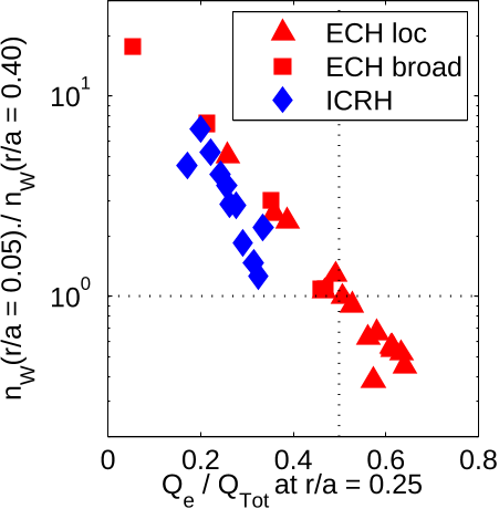 Figure 7. Peaking factor of the W density in the core as a function of the electron heat flux fraction inside r/a = 0.25
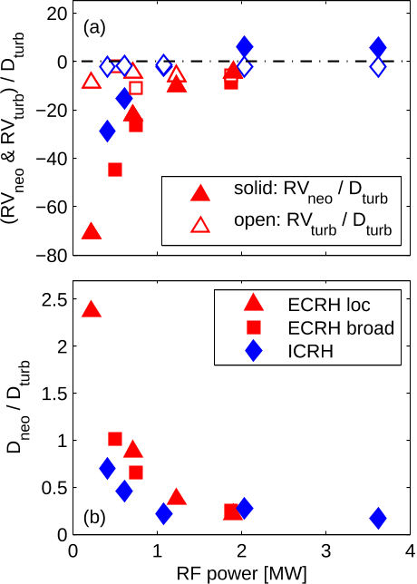 Figure 10. Predicted ratios of the neoclassical and turbulent convection to the turbulent diffusion (a) and ratio of the neoclassical diffusion to the turbulent diffusion (b) in the radial window 0.2 ≤ r/a ≤ 0.3 as a function of the experimental additional RF heating power in MW. Neoclassical and turbulent transport coefficients have been computed by NEO and GKW respectively, and turbulent transport levels have been determined by assuming that the GKW effective heat conductivity matches the power balance anomalous effective heat conductivity computed by TRANSP.
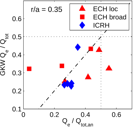 Figure 13. Fraction of the electron heat flux predicted by linear GKW calculations compared to TRANSP power balance
![Figure 9. Experimental peaking factors of W density (already plotted in Fig. 7, full symbols) are compared to the results from the simple model Eq. 1 in open symbols, in (a) with constant Dturb/χeff = 0 (red), 0.1 (green), 1 (blue), in (b) with Dturb/χeff which fits the theoretical results of [22] as a function of Qe/Qi (black)](/figures/figure-9-experimental-peaking-factors-of-w-density-already-1hqnll5l.png) Figure 9. Experimental peaking factors of W density (already plotted in Fig. 7, full symbols) are compared to the results from the simple model Eq. 1 in open symbols, in (a) with constant Dturb/χeff = 0 (red), 0.1 (green), 1 (blue), in (b) with Dturb/χeff which fits the theoretical results of [22] as a function of Qe/Qi (black)
Figure 9. Experimental peaking factors of W density (already plotted in Fig. 7, full symbols) are compared to the results from the simple model Eq. 1 in open symbols, in (a) with constant Dturb/χeff = 0 (red), 0.1 (green), 1 (blue), in (b) with Dturb/χeff which fits the theoretical results of [22] as a function of Qe/Qi (black)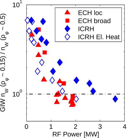 Figure 5. Ratio of central to peripheral W density measured by GIW as a function of the total RF heating power for phases with additional central localized ECRH (triangles), central broad ECRH (squares) and central ICRH (diamonds). The same ICRH phases are also represented in terms of the electron heating fraction of the ICRH power (open diamonds).
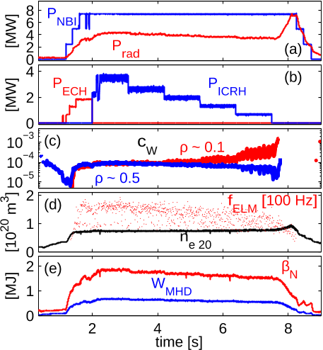 Figure 1. Time traces of AUG shot ♯32404 with decreasing steps of ICRH power, total NBI and radiated powers (a), total ECH and ICRH powers (b), W concentration cW = nW /ne at ρ ≃ 0.1 and ρ ≃ 0.5 (c), ELM frequency and line averaged density (d), normalized β and total stored energy (e).
 Figure 2. Time traces of AUG shot ♯32408 with decreasing steps of ECRH power, total NBI and radiated powers (a), total ECH and ICRH powers (b), W concentration cW = nW /ne at ρ ≃ 0.1 and ρ ≃ 0.5 (c), ELM frequency and line averaged density (d), normalized β and total stored energy (e).
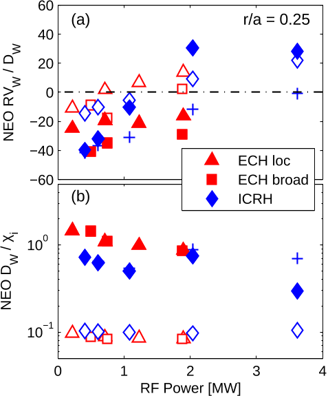 Figure 8. Transport coefficients at r/a = 0.25 computed by NE0 with (full) and without (open) poloidal asymmetries of the W densities. Crosses (’+’) show results with centrifugal effects only for the ICRH cases (impact of ICRH H minority is neglected).
 Figure 6. Normalized logarithmic ion temperature and electron temperature gradients (R/LTi (a) and R/LTe (b) respectively) as well as normalized logarithmic density gradients R/Ln (c) and simple neoclassical impurity peaking parameter R/Ln − 0.5R/LTi (d), electron to ion temperature ratio Te/Ti (e) and thermal Mach number of Deuterium MD = vφ/vthD (f) averaged in the radial window 0.1 ≤ r/a ≤ 0.4 and plotted as a function of the RF heating power in MW. Dashed lines identify the trajectories of discharges ♯32404 and ♯32408 presented in Figs. 1 and 2 respectively.
 Figure 12. Same as Fig. 7, compared with the prediction of combined NEO and GKW linear calculations (open symbols).


![Figure 4. Power density (a) and integrated power (b,c) profiles with localized and broad ECRH (TORBEAM) [45] and with ICRH (TORIC-SSFPQL) [46] as well as NBI (TRANSP) normalized to the maximum power density in (a) and normalized to the total injected power in (b), in actual MW in (c). In (c) the phases with maximum heating power of ECRH (1.9 MW) and ICRH (3.4 MW) are considered. Different x–axis are used in (a,b) and in (c).](/figures/figure-4-power-density-a-and-integrated-power-b-c-profiles-2stqorh3.webp)


![Figure 9. Experimental peaking factors of W density (already plotted in Fig. 7, full symbols) are compared to the results from the simple model Eq. 1 in open symbols, in (a) with constant Dturb/χeff = 0 (red), 0.1 (green), 1 (blue), in (b) with Dturb/χeff which fits the theoretical results of [22] as a function of Qe/Qi (black)](/figures/figure-9-experimental-peaking-factors-of-w-density-already-1hqnll5l.webp)


