
All figures (30)
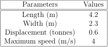 Table 1: Specifications of Springer
 Figure 6: General architecture of USV operation in a maritime environment (Campbell and Naeem, 2012)
 Figure 23: Comparison of computational time to determine path obtained for currents moving with intensity of 1.4 m/s in anticlockwise (AC) and clockwise (C) directions. The interval on each bar denotes the standard deviation of the computational time.
 Figure 24: Comparison of paths obtained for currents moving with intensity of 2.5 m/s in (a) anti-clockwise and (b) clockwise direction. The start and goal states are same as shown in Fig.12. The safety distance constraint of 20 pixels is maintained for both scenarios.
 Figure 26: Comparison of computational time to determine path obtained for currents moving with intensity of 2.5 m/s in anticlockwise (AC) and clockwise (C) directions. The interval on each bar denotes the standard deviation of the computational time.
 Figure 25: Comparison of path length obtained for currents moving with intensity of 2.5 m/s in anticlockwise (AC) and clockwise (C) directions. The interval on each bar denotes the standard deviation of the path length.
 Figure 9: Binary Map with Start and Goal States
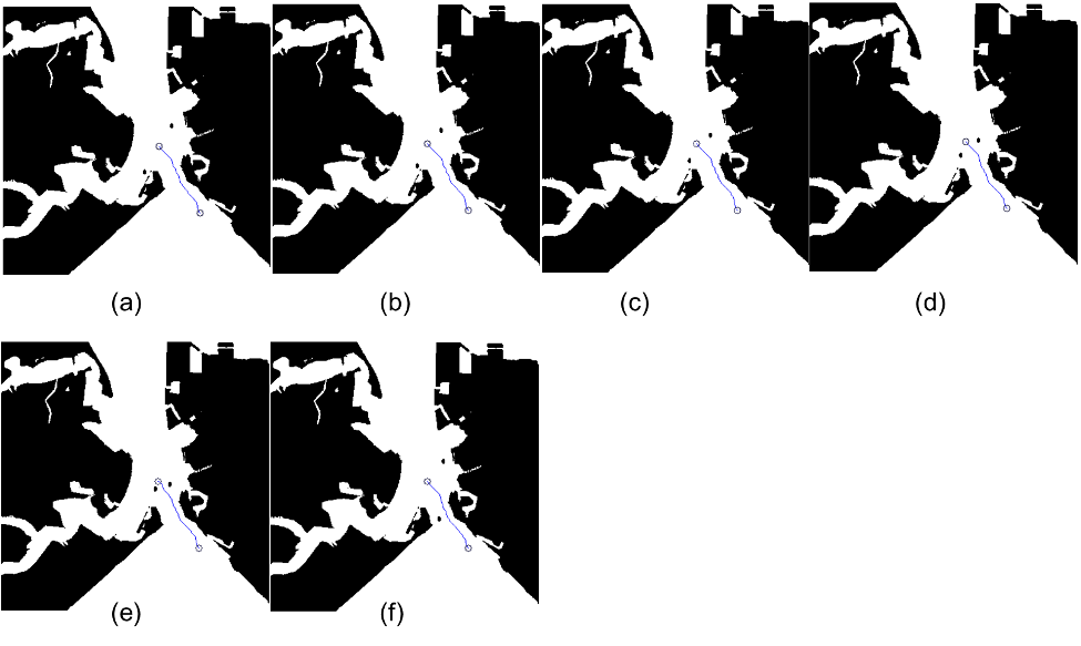 Figure 18: Comparison of paths obtained with different start time (a) 0 (b) 10 (c) 20 (d) 30 (e) 40 (f) 100 seconds. A safety distance constraint of 20 pixel is maintained for all scenarios in the figure.Position of both moving obstacles is plotted at each start time on the binary map, based on the velocity and direction mentioned in Fig.13.
 Figure 2: A schematic showing the path generated by a conventional grid based path planner compared against the path generated by a grid based path planner by considering safety distance and sea surface currents (clockwise). In case of anti clockwise currents, the sea surface currents push the USV towards the obstacle and the proposed algorithm makes sure that a safety distance is maintained to ensure no collision
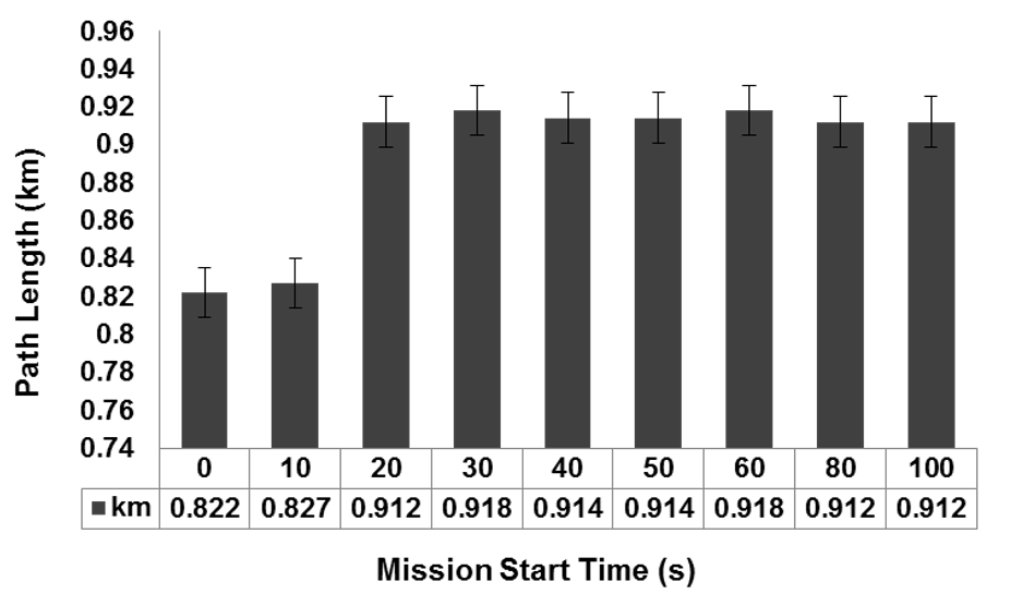 Figure 29: Comparison of path length obtained for scenario with sea surface currents of 1.4 m/s moving in anti-clockwise direction having a moving obstacle for different start time of 0, 10, 20, 30, 40, 50, 60, 80 and 100 seconds. The interval on each bar denotes the standard deviation of the path length.
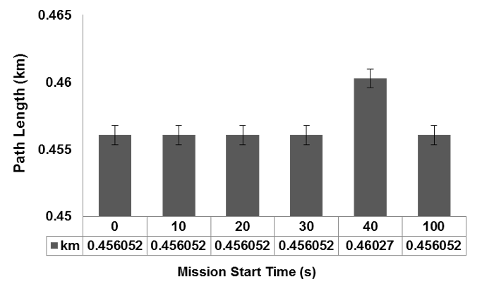 Figure 19: Comparison of path length obtained with different start time 0, 10, 20, 30, 40 and 100 seconds.The interval on each bar denotes the standard deviation of the path length
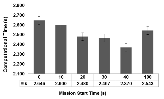 Figure 20: Comparison of computational time obtained with different start time of 0, 10, 20, 30, 40 and 100 seconds. The interval on each bar denotes the standard deviation of the computational time
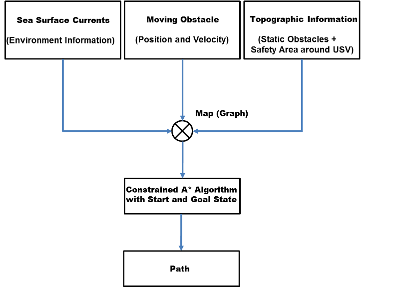 Figure 8: Schematic of the proposed path planning system
 Figure 14: Dimension of the elliptical domain representing the encapsulation of a moving obstacle in a static one in the binary map. The dimensions of ellipse are chosen in accordance with the dimensions of high speed craft having operational velocity range from 6 to 9 knots
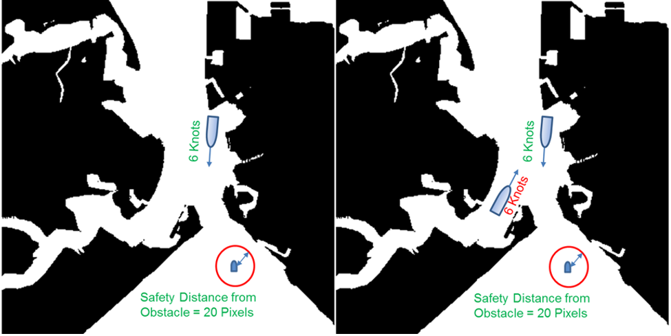 Figure 13: Binary map of the simulation area (Portsmouth harbour) showing velocity and direction of moving obstacles. In this study, 20 pixels has been chosen as the safety distance around an USV.
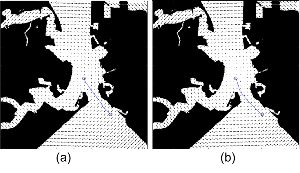 Figure 21: Comparison of paths obtained for currents moving with intensity of 1.4 m/s in (a) anti-clockwise and (b) clockwise direction. The start and goal states are same as shown in Fig.12. The safety distance constraint of 20 pixels is maintained for both scenarios.
 Figure 28: Comparison of paths obtained for scenario with sea surface currents of 1.4 m/s moving in anticlockwise direction having a moving obstacle for different start time of (a) 0 (b) 10 (c) 20 (d) 30 (e) 40 (f) 50 (g) 60 (h) 80 (i) 100 seconds. The start and goal states are same as shown in Fig.12. The safety distance constraint of 15 pixels is maintained for all scenarios.
 Figure 3: Path planning abstraction for USVs (Singh et al., 2016)
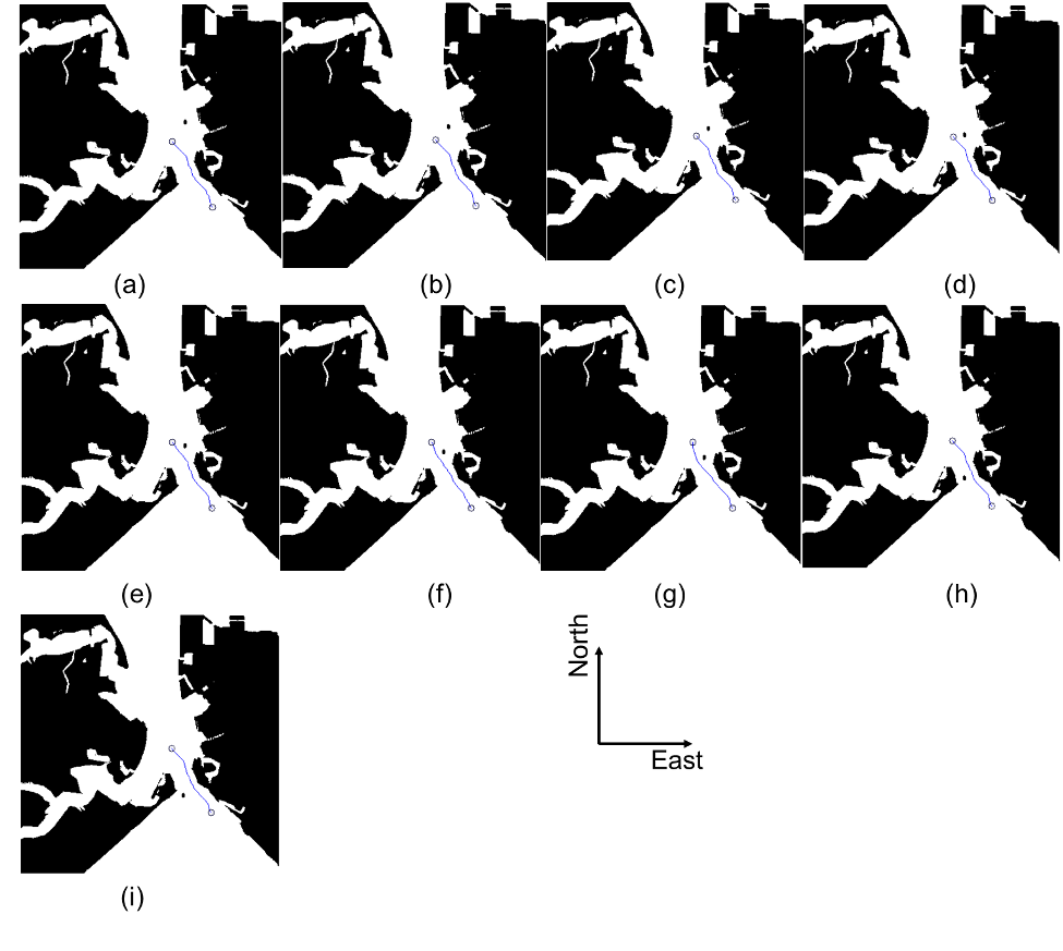 Figure 15: Comparison of paths obtained with different start time (a) 0 (b) 10 (c) 20 (d) 30 (e) 40 (f) 50 (g) 60 (h) 100 (i) 120 seconds. Position of the single moving obstacle is plotted at each start time on the binary map, based on the velocity and direction mentioned in Fig.13
 Figure 11: Resultant path with safety distance of (a) 0 (b) 10 (c) 20 (d) 30 (e) 40 pixels
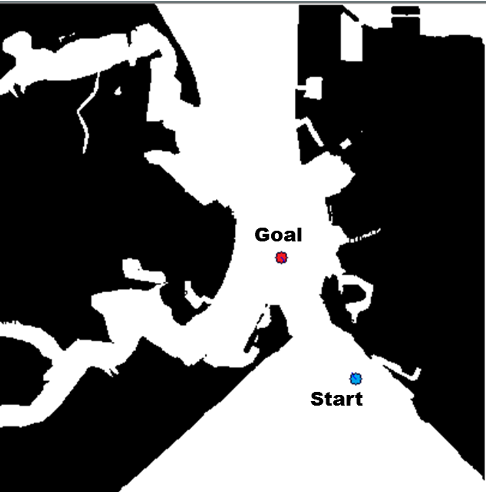 Figure 12: Binary map with start and goal states for simulating A* approach under static and partially dynamic environment
 Figure 7: PID autopilot with a LOS projection algorithm for way-point tracking (Modified from Fossen et al. (2003))
 Figure 27: Comparison of computational time obtained for scenario with sea surface currents of 1.4 m/s moving in anti-clockwise direction having a moving obstacle for different start time of 0, 10, 20, 30, 40, 50, 60, 80 and 100 seconds. The interval on each bar denotes the standard deviation of the computational time.
 Figure 22: Comparison of path length obtained for currents moving with intensity of 1.4 m/s in anticlockwise (AC) and clockwise (C) directions. The interval on each bar denotes the standard deviation of the path length.
 Figure 4: Satellite image of Portsmouth Harbour and its corresponding binary image (Source: Google Maps)
 Figure 5: Schematic of 4-connectivity and 8-connectivity in Cspace
 Figure 16: Comparison of path length obtained with different start time (a) 0 (b) 10 (c) 20 (d) 30 (e) 40 (f) 50 (g) 60 (h) 100 (i) 120 seconds. A safety distance constraint of 20 pixel is maintained for all scenarios in the figure. The interval on each bar denotes the standard deviation of the path length
 Figure 17: Comparison of computational time obtained with different start time (a) 0 (b) 10 (c) 20 (d) 30 (e) 40 (f) 50 (g) 60 (h) 100 (i) 120 seconds. The interval on each bar denotes the standard deviation of the computational time
 Figure 1: The Springer USV
 Figure 10: Compared computational time of A* approach with and without safety distance constraint. The interval on each bar denotes the standard deviation of the computational time


