All figures (9)
![Table 2. Diffusion constants and baseline ECS concentrations for the ion species considered, with values as in [4]. All ion constants were modified as ~Dk ¼ Dk=l 2 , where λ = 1.6 is the tortuosity. The general anion X− was given the properties of Cl−.](/figures/table-2-diffusion-constants-and-baseline-ecs-concentrations-2je1r9ai.png) Table 2. Diffusion constants and baseline ECS concentrations for the ion species considered, with values as in [4]. All ion constants were modified as ~Dk ¼ Dk=l 2 , where λ = 1.6 is the tortuosity. The general anion X− was given the properties of Cl−.
Table 2. Diffusion constants and baseline ECS concentrations for the ion species considered, with values as in [4]. All ion constants were modified as ~Dk ¼ Dk=l 2 , where λ = 1.6 is the tortuosity. The general anion X− was given the properties of Cl−. Fig 1. Model system of a 3-D cylinder of ECS containing a morphologically detailed neuron. (A) The simulated domain is denoted by O, and the boundary is denoted by @O. Exchange of ions between the neuron and ECS was modeled as a set of point sources (marked by blue dots). Two measurement points were used to create time series in the Results-section. These are shown as the green and purple points. (B) Each point source was included as a sink/ source of each ion species, as well as a capacitive current.
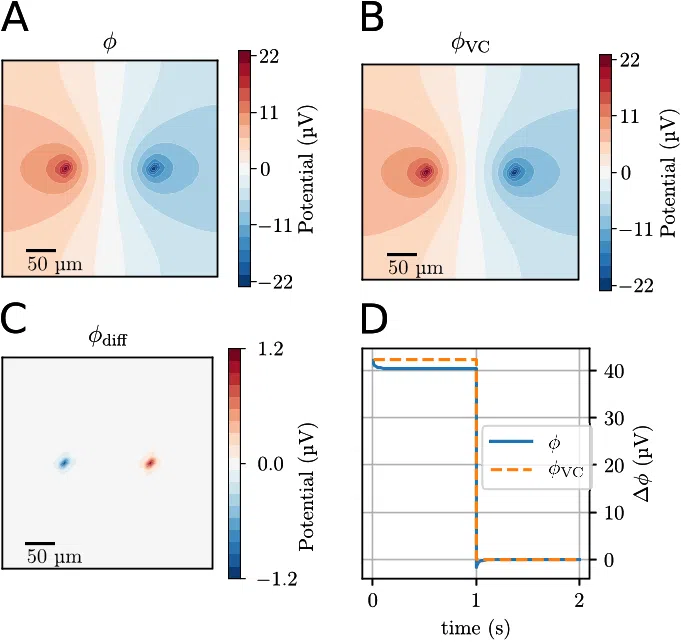
 Fig 3. Application with a K+ point source/sink pair in a 3-D box containing a standard ECS ion solution. The source and sink were turned on at t = 0 s, and turned off at t = 1 s. The simulation was stopped at t = 2 s. (A) The total electrical potential ϕ at the end of the stimulus period (t = 1.0 s) in a plane intersecting the source and sink. (B) The volume conductor component of the electrical potential, ϕVC. (C) The diffusive component of the electrical potential ϕdiff. (D) The difference in the electric potential between points close to the point sources (blue line), also shown is the differences in the VC component of the potential (stapled yellow line). Δϕ is defined as Δϕ = ϕ(xleft) − ϕ(xright), where xleft and xright were points 5 μm away from the left and right, respectively (see Methods).
 Fig 6. Spatial profile of the ECS potential at a selected time point. The ECS potential was averaged over a 100 ms interval between t = 79.9 s and 80 s. This averaging low-pass filters the potential. (A) ECS potential as predicted by the KNP-scheme. (B) The VC component of the potential. (C) The diffusive component of the potential.
 Fig 2. Electrodiffusion in a simple 1-D system containing no current sources. The system had an initial step concentration of NaX being 140 mM for x< 0 and 150 mM for x> 0. (A) Dynamics of the potential difference between the left and right sides of the system on a short timescale. Δϕ is defined as Δϕ = ϕ(xright) − ϕ(xleft), where xright = 0.1 μm and xleft = −0.1 μm. In PNP simulations, the system spent about 10 ns building up the potential difference across the system. In KNP simulations, the steady-state potential was assumed to occur immediately. After 10 ns, the schemes were virtually indistinguishable. (B) Dynamics of the potential between xright = 50 μm and xleft = −50 μm on a long timescale. The PNP- and KNP-schemes gave identical predictions. (C) The concentration profiles in the system at t = 1.0 s as obtained with KNP, DO and according to the theoretical approximation when NaX develops as a single concentration moving by diffusion with a modified diffusion coefficient.
 Fig 5. Ion concentration dynamics at selected measurement points. The locations of the measurement points were in the ECS near the soma (green) and apical dendrites (purple) of the neuron. Δc(t) is the change in concentration from the initial value, defined as Δc(t) = c(t) − c(0). (A)-(B) Dynamics of all ion species as predicted by the KNPscheme. (C)-(F) A comparison between the KNP and DO predictions at the measurement point near the soma. (G)-(J) A comparison between the KNP and DO predictions at the measurement point near the apical dendrites. (C)-(J) To
 Fig 7. Dynamics of the ECS potential at selected measurement points. The selected measurement points were in the ECS near the soma (green) and apical dendrites (purple) of the neuron. (A)-(B) Dynamics of the ECS potential for the first 80 s of the simulation. Each data point represent an average over a 100 ms time interval, which effectively low-pass filtered the signal. (C)-(D) High resolution time series for the ECS potential during a neural AP. The data were not low-pass filtered, but had a temporal resolution of 0.1 ms.
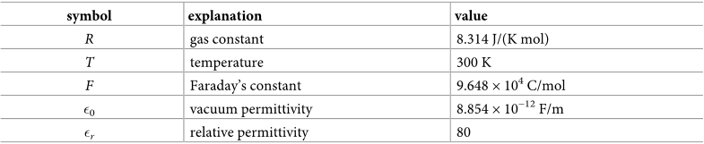 Table 1. The physical parameters used in the simulations.
 Fig 4. (A)-(D)The change in ionic concentration for Ca2+, K+, Na+, and X−, respectively, as measured at t = 80 s, compared to the initial concentration. Δck is the change in concentration from the initial value, defined as Δck = ck(t) − ck(0). The concentrations were measured in a 2-D slice going through the center of the computational mesh, and the neuron morphology was stenciled in. The green and purple dots signify selected measurement points in the ECS near the soma (green) and apical dendrites (purple) of the neuron, which are reference points for the analysis in the following sections.
![Table 2. Diffusion constants and baseline ECS concentrations for the ion species considered, with values as in [4]. All ion constants were modified as ~Dk ¼ Dk=l 2 , where λ = 1.6 is the tortuosity. The general anion X− was given the properties of Cl−.](/figures/table-2-diffusion-constants-and-baseline-ecs-concentrations-2je1r9ai.webp)