
All figures (14)
 Fig. 11. H-plane filter optimal coarse-model response (—), and the HFSS (fine-model) response: (a) at the initial solution ( ) and (b) at the SMIS algorithm solution reached after three iterations ( ).
 TABLE IV OPTIMIZABLE PARAMETER VALUES OF THE SIX-SECTION H-PLANE WAVEGUIDE FILTER
 TABLE III OPTIMIZATION METHODS USED ON THE SEVEN-SECTION CAPACITIVELY LOADED IMPEDANCE TRANSFORMER
![Fig. 10. Six-section H-plane waveguide filter [7]. (a) Physical structure. (b) Coarse model as implemented in MATLAB .](/figures/fig-10-six-section-h-plane-waveguide-filter-7-a-physical-1bz72gq2.png) Fig. 10. Six-section H-plane waveguide filter [7]. (a) Physical structure. (b) Coarse model as implemented in MATLAB .
Fig. 10. Six-section H-plane waveguide filter [7]. (a) Physical structure. (b) Coarse model as implemented in MATLAB .![Fig. 1. Error plots for a two-section capacitively loaded impedance transformer [4] exhibiting the quasi-global effectiveness of SM (light grid) versus a classical Taylor approximation (dark grid). See text.](/figures/fig-1-error-plots-for-a-two-section-capacitively-loaded-3dqus87x.png) Fig. 1. Error plots for a two-section capacitively loaded impedance transformer [4] exhibiting the quasi-global effectiveness of SM (light grid) versus a classical Taylor approximation (dark grid). See text.
Fig. 1. Error plots for a two-section capacitively loaded impedance transformer [4] exhibiting the quasi-global effectiveness of SM (light grid) versus a classical Taylor approximation (dark grid). See text.![Fig. 2. Error plots for a two-section capacitively loaded impedance transformer [4] exhibiting the quasi-global effectiveness of SM-based interpolating surrogate, which exploits OSM (light grid) versus a classical Taylor approximation (dark grid). See text.](/figures/fig-2-error-plots-for-a-two-section-capacitively-loaded-2uki65k7.png) Fig. 2. Error plots for a two-section capacitively loaded impedance transformer [4] exhibiting the quasi-global effectiveness of SM-based interpolating surrogate, which exploits OSM (light grid) versus a classical Taylor approximation (dark grid). See text.
Fig. 2. Error plots for a two-section capacitively loaded impedance transformer [4] exhibiting the quasi-global effectiveness of SM-based interpolating surrogate, which exploits OSM (light grid) versus a classical Taylor approximation (dark grid). See text. Fig. 3. Illustration of the SMIS concept. The aim is to calibrate the mapped coarse model (the surrogate) to match the fine model using different input and output mappings for each sampled response.
 Fig. 4. Seven-section capacitively loaded impedance transformer: “Fine” model.
 Fig. 5. Seven-section capacitively loaded impedance transformer: “Coarse” model.
 Fig. 6. Seven-section capacitively loaded impedance transformer: optimal coarse-model response (- -), the optimal minimax fine-model response (—), and the fine-model response at the initial solution or at the optimal coarse-model solution ( ).
 TABLE II OPTIMIZABLE PARAMETER VALUES OF THE SEVEN-SECTION CAPACITIVELY LOADED IMPEDANCE TRANSFORMER
 Fig. 7. Seven-section capacitively loaded impedance transformer: optimal coarse-model response (- -), the optimal minimax fine-model response (—), and the fine-model response at the SMIS algorithm solution obtained after five iterations (six fine-model evaluations) ( ).
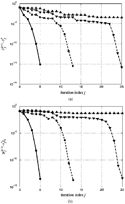 Fig. 8. (a) First 25 iterations of the difference between the fine-model objective function U obtained using the SMIS algorithm ( ) and the fine-model objective function at the fine-model minimax solution U obtained by the Hald–Madsen algorithm ( ), the HASM surrogate optimization algorithm using exact gradients (r), and the HASM surrogate optimization algorithm using the Broyden update ( ). (b) The corresponding difference between the designs.
 Fig. 9. (a) Difference between the fine-model objective function U obtained using the SMIS algorithm ( ) and the fine-model objective function at the fine-model minimax solution U obtained by the Hald–Madsen algorithm ( ), the HASM surrogate optimization algorithm using exact gradients (r), and the HASM surrogate optimization algorithm using the Broyden update ( ). (b) The corresponding difference between the designs.


![Fig. 10. Six-section H-plane waveguide filter [7]. (a) Physical structure. (b) Coarse model as implemented in MATLAB .](/figures/fig-10-six-section-h-plane-waveguide-filter-7-a-physical-1bz72gq2.webp)
![Fig. 1. Error plots for a two-section capacitively loaded impedance transformer [4] exhibiting the quasi-global effectiveness of SM (light grid) versus a classical Taylor approximation (dark grid). See text.](/figures/fig-1-error-plots-for-a-two-section-capacitively-loaded-3dqus87x.webp)
![Fig. 2. Error plots for a two-section capacitively loaded impedance transformer [4] exhibiting the quasi-global effectiveness of SM-based interpolating surrogate, which exploits OSM (light grid) versus a classical Taylor approximation (dark grid). See text.](/figures/fig-2-error-plots-for-a-two-section-capacitively-loaded-2uki65k7.webp)


