
All figures (17)
 Table 1 Parameters Used to Generate the Fictitious Model Atmosphere and Spectrum
 Figure 6. Marginalized posterior probability distributions for each of the retrieved gases (rows) and observational scenario (columns). In each panel, the probability distribution for each retrieval technique are shown in different colors. The Gaussian probability distributions from optimal estimation are in red, differential evolution Markov chain Monte Carlo in blue, and bootstrap Monte Carlo in green. The priors for each gas are the dot-dashed red curve. The true answer is the vertical black line. (A color version of this figure is available in the online journal.)
 Table 3 Numerical Summary of the Retrieval Results for Several Parameters as Derived from Each Retrieval Technique and Observational Scenario
 Figure 2. Synthetic planet atmosphere and spectrum. Top left: model temperature–pressure profile. The solid curve is the temperature profile and the dashed curve is the averaged thermal emission contribution function, or where the emission in the atmosphere is coming from. The temperature profile is constructed using Equations (13)–(16) and the parameters in Table 1. Top right: thermal emission contribution function. This plot shows where the emission is coming from as a function of wavelength, smoothed to a resolution of 0.05 μm. Red corresponds to the peak of the thermal emission weighting functions, where the optical depth is unity, and blue represents zero emission. Most emission emanates between a few bars and 0.01 bars with deeper layers probed by shorter wavelengths. Bottom left: resulting spectrum smoothed to a resolution of 0.05 μm. Blackbodies for the hottest, coolest, and average temperatures are shown. The dotted curves at the bottom are the filter profiles for typical photometric observations. Bottom right: gas Jacobian generate from Equation (9). This plot shows the sensitivity of the flux contrast as a function of wavelength to the various absorbers (the units are arbitrary but consistent).
 Figure 5. Fits to the three different sets of data (columns) from each of the three different retrieval techniques (rows). The first scenario consists of the four IRAC photometry channels. The second scenario consists of the four IRAC photometry channels, ground-based H- and Ks-band photometry, and HST WFC3 spectroscopy. The third scenario is representative of a FINESSE-like future, spaceborne telescope. The best fits from each scenario and technique are shown in light blue. The light-blue circles with the black borders are the best fits binned to the data. The chi-squared per data point from the optimal estimation best-fit broadband scenario, multi-instrument scenario, and future telescope scenario are, respectively, 0.197, 0.686, and 0.955. The bootstrap Monte Carlo and the differential evolution Markov chain Monte Carlo approaches generate many thousands of spectra. The median of these spectra is shown in blue and the 1σ and 2σ spread in the spectra are shown in dark- and light-red, respectively. The best fit from the thousands of spectra are shown in light blue. The best-fit reduce-chi-squares from BMC and DEMC are of similar values to those from OE. The dotted curves at the bottom of each panel are the broadband filter transmission functions. The insets are a zoom in of a spectral region between 1 and 2 μm to better show the spread in the spectra. Note that there is virtually no spread in the spectra for the future telescope case.
 Figure 9. Temperature profile posteriors for each observational scenario (columns) and each retrieval technique (rows). The solid black curve in each panel is the true temperature profile constructed with Equations (13)–(16) and the parameters in Table 1. The dashed black curve is constructed from the temperature parameters, xa, just as in Figure 4. The blue curve is the median temperature profile. The light blue curve in each panel is the best-fit temperature profile for the corresponding scenario and technique. The dark and light red regions are the 1σ and 2σ (68% and 95%) uncertainties, respectively.
 Figure 12. Marginalized posterior probability distributions for each of the retrieved gases (rows) and observational scenario (columns) using the Level-by-Level temperature profile approach. In each panel, the posteriors for optimal estimation (red) and bootstrap Monte Carlo (green) are shown. The Gaussian priors for each gas are shown with the dot-dashed red curve. The true answer is the vertical black line.
 Figure 8. Marginalized posterior probability distributions for each of the retrieved temperature parameters (rows) and observational scenario (columns). In each panel, the probability distribution for each retrieval technique are shown in different colors. The Gaussian probability distributions from optimal estimation are in red, differential evolution Markov chain Monte Carlo in blue, and bootstrap Monte Carlo in green. The priors for each gas are the dot-dashed red curve. The true answer is the vertical black line.
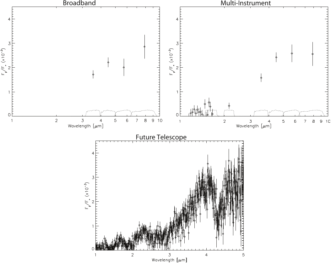 Figure 3. Spectrum of the synthetic hot Jupiter observed in three different scenarios. These “observations” are created by convolving the high-resolution spectrum in Figure 1 with the appropriate instrumental profiles. Random noise is then added to each data point. Top left: synthetic observations as viewed through the Spitzer broadband 3.6, 4.5, 5.7, and 8 μm channels. Top right: multi-instrument observations that include WFC3 (1.15–1.63 μm), ground-based H and Ks, and Spitzer broadband (3.6, 4.5, 5.7, and 8 μm). Bottom: hypothetical future spaceborne observations. The dotted curves on the bottom of each plot are the photometric transmission functions.
 Figure 13. Temperature profile posteriors using the Level-by-Level temperature profile approach for each observational scenario (columns) and two of the retrieval technique (rows). The solid black curve in each panel is the true temperature profile constructed with Equations (13)–(16) and the parameters in Table 1. The blue curve is the median temperature profile. The dashed black curve is the prior temperature profile constructed from xa, as in Figure 4. The prior widths for each level (not shown) are ±400 K. The dark and light red regions are the 1σ and 2σ (68% and 95%) uncertainties, respectively. The green curve is the averaging kernel profile for temperature. The atmospheric regions over which this is a maximum is where we can retrieve temperature information with less dependence on the prior (see text). (A color version of this figure is available in the online journal.)
 Figure 11. Fits to the three different sets of data (columns) from two of the retrieval techniques (rows) using the Level-by-Level temperature approach. The best fits are shown in light blue. The optimal estimation best fit in each observational scenario is the global best fit. The light-blue circles with a black border are the best-fit spectra binned to the data. The chi-squared per data point values for the broadband, multi-instrument, and future telescope scenarios are, respectively, 0.155, 0.665, and 0.948. The bootstrap Monte Carlo approach generates many thousands of spectra. The median of these spectra is shown in blue and the 1σ and 2σ spread in the spectra are shown in dark- and light-red, respectively. The dotted curves at the bottom of each panel are the broadband filter transmission functions.
 Figure 7. Gas correlations for each of the observing scenarios. The red curves in each are the analytic confidence intervals from the optimal estimation posterior covariance matrix (Ŝ). The inner ellipses are the 1σ (68%) and the outer ellipses are the 2σ (95%) confidence interval. The 1σ and 2σ confidence intervals derived from the differential evolution Markov chain Monte Carlo are shown in dark and light blue, respectively. Note that the scales for the confidence intervals derived from the broadband observations (top) and the multi-instrument observations (middle) are the same. The scale on the future telescope (bottom) confidence intervals is much smaller.
 Table 2 Gaussian Prior Parameter Values and Widths
 Figure 4. Temperature and gas priors (inset). Dark red represents the 1σ spread in the allowed temperature profiles as a result of the prior parameter distributions in Table 2. Light red is the 2σ spread allowed in the temperature profiles. The blue curve is the median temperature profile and the black curve is the temperature profile constructed from xa in Table 2. The gas priors are broad Gaussians. H2O and CO have the same prior mean, CH4 and CO2 have the same prior mean. Note that the prior is Gaussian in log of the mixing ratios. The y-axis on the inset is normalized probability.
 Figure 14. Effect of three different Level-by-Level temperature profile priors on the retrieved temperatures (top) and spectra (bottom). The different temperature profile priors are shown as the colored dashed curves. The prior widths (not shown) at each level are ±400 K, similar to those in Figure 13. The resultant retrieved profiles are shown as the solid colored curves. The thick black curve is the true temperature profile. The solid gray region is the 1σ confidence interval from the retrievals in Figure 13. Note how the retrieved profiles all converge within the 1σ confidence interval regardless of the temperature prior. The best agreement is in the middle atmosphere where the thermal emission weighting functions are a maximum, and hence the averaging kernel profiles from Figure 13 are also a maximum. The spectra in the second row illustrate the effects of the different retrieved temperature profiles of corresponding color. There is virtually no difference in the resultant spectra for high-quality data. The dotted curves at the bottom are the broadband filter functions.
 Figure 1. Comparison of the thermal emission spectrum from our forward model (black) with the NEMESIS forward model (red). The temperature–pressure profile is shown in the inset. For this comparison we assume uniform mixing ratios of 10−4 for CH4, CO2, CO, and H2O. H2 is set to 0.85 and He is set to 0.15. This planet is assumed to be hydrogen dominated (mean molecular weight of 2.3 amu) with a radius of 1 RJ , a gravity of 22 ms−2, orbiting a 5700 K pure blackbody star with a radius of 1 Rsun.
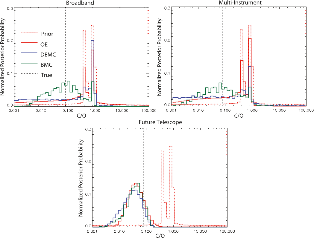 Figure 10. C to O ratio posteriors. The dot-dashed red curve is the prior, the solid red curve is from OE, blue is from DEMC, and green is from BMC. The vertical dashed line is the true C/O. In the top left panel are the C/O’s derived from the broadband observational scenario, in the top right are the C/O’s derived from the multi-instrument scenario, and in the bottom are the C/O’s derived from the future spaceborne telescope scenario. Though it appears that the BMC characterizes the C/O errors well, it is for the wrong reasons. See Section 3.3.3.


