


A TIME-FREQUENCY APPROACH TO BLIND DECONVOLUTION
IN MULTIPATH UNDERWATER CHANNELS
N. Martins, S. Jesus
∗
SiPLAB–FCT, University of Algarve
Campus de Gambelas, 8000 Faro, Portugal
nmartins@ualg.pt, sjesus@ualg.pt
C. Gervaise, A. Quinquis
EIA Dpt., ENSIETA
29806 Brest Cedex 09, France
gervaice@ensieta.fr, quinquis@ensieta.fr
ABSTRACT
Blind deconvolution is presented in the underwater acoustic
channel context, by time-frequency processing. The acous-
tic propagation environment was modelled as a multipath
propagation channel. For noiseless simulated data, source
signature estimation was performed by a model-based me-
thod. The channel estimate was obtained via a time-fre-
quency formulation of the conventional matched-filter. Si-
mulations used a ray-tracing physical model, initiated with
at-sea recorded environmental data, in order to produce rea-
listic underwater channel conditions. The quality of the
estimates was 0.793 for the source signal, and close to 1
for the resolved amplitudes and time-delays of the impulse
response. Time-frequency processing has proved to over-
come the typical ill-conditioning of single sensor determi-
nistic deconvolution techniques.
1. INTRODUCTION
Two fundamental problems arising in many signal proces-
sing applications are channel and source signature estima-
tion, often referred as deconvolution. Areas such as data
transmission, reverberation cancellation, seismic signal pro-
cessing, image restoration, etc., are some examples where
deconvolution finds application. One of these areas is ocean
acoustics, where a fundamental problem is the passive cha-
racterization of acoustic transients and the ocean environ-
ment. This paper aims to give an approach to solve the
problem of blind deconvolution in ocean acoustics, i.e., ob-
taining at once estimates of the emitted signal and the me-
dium impulse response (IR) representative of its physical
properties. In view of the typical structure of underwater
channel model-IRs, constituted by a set of close arrivals,
time-frequency (TF) distributions (TFDs) have been chosen
as a mean for separating the various replicas of the typically
transient source signal. A shallow-water realistic scenario
was chosen to support the presentation.
∗
Thanks to MCT, FCT, PRAXIS XXI (BM/19298/99) for funding, and
to Profs. A. Quinquis and C. Gervaise for the favourable reception at EN-
SIETA.
2. MATHEMATICAL BACKGROUND
One of the main mathematical tools essential in the present
work is the Wigner-Ville distribution (WV), defined by[1]
WV
x
(t, f)=
∞
−∞
x
t +
τ
2
x
∗
t −
τ
2
e
−j2πfτ
dτ,
(1)
where
∗
designates complex conjugate. An also important
TFD is the signal-dependent distribution radially Gaussian
kernel distribution (RGK)[2]
RGK
x
(t, f)=IFT2[Φ
RGK,x
(ν, τ )AF
x
(ν, τ )] , (2)
where Φ
RGK,x
(t, f), the kernel of the distribution, is adap-
ted to the signal to be analyzed, AF
x
(ν, τ ) stands for the
ambiguity function of x(t), and IFT2[·] designates the bi-
-dimensional (2D) inverse Fourier transform operator. Sig-
nal reconstruction was performed via an inverse TF trans-
formation. The basis method[3] was employed, where a
linear combination of the basis functions e
k
(t) was used to
obtain the final source signal estimate such as
ˆs(t)=
N
b
k=1
α
k
e
k
(t). (3)
The functions e
k
(t) span the signal space to which the esti-
mate is confined. Channel estimation was performed taking
into account the TF formulation of the matched-filter (MF).
The fact that the WV obeys to Moyal’s formula[4] conduces
to the following equation:
∞
−∞
WV
x
1
(t, f)WV
∗
x
2
(t+τ ),x
2
(t)
(t, f) dt df =
∞
−∞
x
1
(t)x
∗
2
(t + τ) dt
∞
−∞
x
1
(t)x
∗
2
(t) dt
∗
. (4)
This shows that temporal correlation can be performed in
the TF domain.
II - 12250-7803-7402-9/02/$17.00 ©2002 IEEE

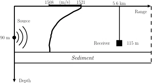
3. SIMULATION RESULTS
The simulated data set corresponds to a canonical two-
-layered shallow-water waveguide whose environment is the
real data acquisition scenario of the INTIMATE ’96 sea
trial[5]. The acoustic source is positioned at 90-m depth,
and the receiver is located at 5.6-km range and 115-m depth,
as illustrated in Fig. 1. The 135-m water column is superim-
Depth
Range
90 m
Source
115 m
Sediment
5.6 km
Receiver
1508
1521
(m/s)
Fig. 1. Scenario of the INTIMATE ’96 sea trial.
posed to a perfectly rigid-modelled bottom. The considered
sound speed profile is shown within Fig. 1. Application of
the ray/beam propagation model BELLHOP[6], taking as
input the environment in Fig. 1, allowed to obtain the refe-
rence channel IR h(t)–Fig. 2. A total number of M =45
0.3 0.4 0.5 0.6 0.7 0.8 0.9
0
0.2
0.4
0.6
0.8
1
Time (s)
Normalized amplitude
Resolved arrivals
Fig. 2. Reference IR h(t) of the canonical scenario. The dashed
line separates unresolved from resolved arrivals.
arrivals have been predicted by the model, spanning the time
interval [0.31, 0.86] s. The amplitudes a
m
and time-delays
τ
m
of the arrivals are the channel parameters to estimate,
grouped into the vectors a and τ , respectively. The source
signal s(t) consists of a T =0.0625-s duration linear fre-
quency modulation (LFM) pulse, spanning the [300, 800]-
Hz instantaneous frequency (IF) range. The IR is split into
2 packets of arrivals: one packet contains the first 8 arrivals,
and the other contains the remaining 37 arrivals, which can
be seen as unresolved and resolved arrivals, respectively.
Unresolved arrivals are adjoint arrivals whose arrival times
differ by less than the inverse of the bandwidth of s(t). The
received signal is modelled by
r(t)=x(t)+ξ(t), (5)
where x(t) and ξ(t) are the signal and noise terms, respec-
tively. Next two sub-sections describe results for noiseless
data, whereas Sec. 4 addresses deconvolution robustness to
noise.
3.1. Source Signature Estimation
Considering the multi-component structure of the noiseless
received signal, source signature estimation was performed
by application of the basis method, whose output is given by
(3), and whose model function was defined by the product
of WV
r
(t, f) by a 2D function, centered on the IF estimate
of s(t). This procedure is an approach to solve a mul-
ti-component signal separation problem, conditioned on the
overlap between the very early arrivals.
The information of the purely phase modulated emitted
signal s(t)=exp [jϕ
i
(t)] is contained in the IF f
i
(t), apart
from a phase term, since the signal’s amplitude modulation
component is constant. This implies that most part of the
signal energy concentrates around the line defined by the
points [t, f
i
(t)], in the TF space[7]. This characteristic mo-
tivated source signal estimation, by a first estimation of the
IF of s(t). Due to the typical presence of one or a few strong
arrivals in h(t), the IF estimation consisted of the global
maximization with respect to t, of the signal-dependent dis-
tribution RGK of the received signal, RGK
r
(t, f):
[t,
ˆ
f
i
(t)] = { (t, f ):t=arg max
t
RGK
r
(t, f),f∈B}. (6)
In RGK
r
(t, f), for an unitary kernel volume, the first 8 ar-
rivals are grouped in a support of large energy, as shown in
Fig. 3. The remaining 37 arrivals, “clustered” in quadruplets,
Fig. 3. Contour plot of the RGK signal-dependent distribution of
the received signal, RGK
r
(t, f).
are clearly distinguished. Maximization of RGK
r
(t, f)
II - 1226

with respect to t, gave rise to an accurate IF estimate[8].
The IF is estimated via maximization of a signal-dependent
TFD, since here, the interference terms (ITs) are quite re-
duced, comparatively to non-signal-dependent TFDs, as the
WV. In that sense, non-signal-dependent TFDs are inappli-
cable in (this) case of signals composed by a sum of repli-
cas, besides the large variance of the estimate, in presence
of noise.
It is likely that the proposed approach will yield a good
IF estimate mainly for the class of purely phase modulated
source signals, for which WV
s
(t, f) is usually concentrated
on a continuous region centered on the line defined by the
pair [t, f
i
(t)]. However, for a non-linear frequency modu-
lation source signal, there are always ITs in its auto-WV,
what may require a smaller value for the kernel volume of
RGK
r
(t, f), if some ITs of that auto-WV have greater am-
plitude than the signal terms. A quadratic IF has been accu-
rately estimated in [9]. The extension to the case of incons-
tant amplitude modulation may hypothetically be treated in
the same manner, provided that the instantaneous amplitude
is a sufficiently smooth function, what weakly increases the
spread of the auto-WV along the IF.
For application of the basis method, the considered sig-
nal space was the subspace of band-limited signals, in the
band [0,f
s
/2], which is a natural choice when dealing with
discrete-time signals. The obtained source estimate is de-
picted in Fig. 4, and corresponds to a cross-correlation coef-
ficient of 0.793 with s(t). The band limitation signal cons-
0.25 0.3 0.35 0.4 0.45
−1
−0.5
0
0.5
1
Time (s)
Normalized amplitude
Fig. 4. Source estimate –real part of ˆs(t).
traint is reflected not only in the increased signal duration,
but also in an increase of the IF range, since the limitation
to [0,f
s
/2] gave the freedom to the estimate’s IF to extend
in the whole [0, 850] Hz interval.
3.2. Channel Estimation
This sub-section describes the estimation of the parameters
{a
m
,τ
m
; m =1, ..., M} that characterize the channel’s
IR, by use of the TF formulation of the MF mentioned in
Sec. 2. For the case of an LFM signal at emission, and
for the particular cases x
1
(t)=r(t) and x
2
(t)=s(t), (4)
is well approximated by the integration of WV
r
(t, f) along
f
i
(t)[8]. Thus, the IF estimate obtained in Sec. 3.1 was used
to do this “coherent integration” of WV
r
(t, f). The obtai-
ned channel estimate is shown in Fig. 5. For the problem at
0 0.1 0.2 0.3 0.4 0.5 0.6
0
0.2
0.4
0.6
0.8
1
Time (s)
Normalized amplitude
Fig. 5. Channel estimate, obtained by coherent integration of
WV
r
(t, f).
hand, it can be verified that the obtained resolution is com-
parable to that of the MF result–Fig. 6. It can be shown
0 0.1 0.2 0.3 0.4 0.5 0.6
0
0.2
0.4
0.6
0.8
1
Time (s)
Normalized amplitude
Fig. 6. Channel estimate obtained by classic matched-filtering.
that the relation between the two resolutions depends on the
relative values of the IF range and the inverse of T [8]. In
practice, the first 8 arrivals of h(t) are not resolved, and the
quality of the channel estimate will refer only to the remai-
ning 37 arrivals. One normalized measure of the quality can
be given as
ρ
a
=1−
||a −
ˆ
a||
2
; ρ
τ
=1−
||τ −
ˆ
τ ||
2
, (7)
where the vectors must first be unitarily normalized. The
quality of the channel estimate is given by ρ
a
=0.9664 and
ρ
τ
=0.9996. The present approach can be applied also to
RGK
r
(t, f).
Alternatively to the procedure of TF coherent integra-
tion, the channel estimate can be obtained by cross-
-correlation between ˆs(t) and r(t), once ˆs(t) be available.
This approach allowed to obtain an estimate very similar to
the previous estimates[8].
4. PERFORMANCE IN NOISE
In this section, the received signal in (5) contains non-zero
white noise ξ(t). Looking at the expected value of
II - 1227

WV
r
(t, f), one finds that
E[WV
r
(t, f)] = WV
x
(t, f)+σ
2
ξ
, (8)
where σ
2
ξ
is the noise variance. It can readily be seen that
the blind deconvolution method can be performed the same
way as in the noiseless data case of Sec. 3, provided that
WV
r
(t, f) is replaced by its expected value. Regarding
RGK
r
(t, f), one can verify that
E[AF
r
(ν, τ )] = AF
x
(ν, τ )+σ
2
ξ
δ(ν)δ(τ ), (9)
hence not representing a significant change on the calculus
of the optimal kernel, relatively to the noiseless case. The
signal-to-noise ratio (SNR) is defined as:
SNR
dB
=10log
1
N
N−1
n=0
s
2
(n)
σ
2
ξ
, (10)
where N is the number of time samples. The empirical mea-
sures below were estimated from 100 trials for each SNR
value. Source estimation performance in noise is illustrated
in Fig. 7, by a plot of the normalized correlation coefficient
as a function of the SNR. Channel estimation performance
−20 −15 −10 −5 0 5 10
0.3
0.4
0.5
0.6
0.7
0.8
0.9
1
SNR (dB)
Normalized correlation coefficient
Fig. 7. Source estimation performance in noise.
in noise was measured by the normalized performance mea-
sures (7), for values of SNR ranging from -5 to 10 dB –
Fig. 8. For values of SNR below -5 dB, it was not techni-
cally possible to clearly distinguish the 37 resolved peaks,
with a fixed threshold.
−5 0 5 10
0.992
0.993
0.994
0.995
0.996
0.997
0.998
0.999
1
SNR (dB)
Performance measure
:
amplitudes
time−delays
:
Fig. 8. Channel estimation performance in noise.
5. CONCLUSIONS AND PERSPECTIVES
This work has shown the feasibility of single sensor blind
deconvolution by TF processing, for a realistic multiple time
delay-attenuation channel, and a deterministic non-stationary
source signal. The simulated data set was based on actual
environmental data recorded at sea during a shallow wa-
ter experiment, leading to a particularly difficult test case,
where there are a high number of closely spaced multipaths.
The deconvolved source signal showed a correlation with
the emitted signal close to 0.8, while the channel parameter
estimation was shown to be effective and robust for SNR as
low as -5 dB. Application of the proposed methods on at-sea
recorded data is being performed at this time.
6. REFERENCES
[1] J. Ville, “Th
´
eorie et applications de la notion de signal
analytique,” C
ˆ
ables et Transmissions, vol. 2A, pp. 61–
74, 1948.
[2] R.G. Baraniuk and D.L. Jones, “A radially Gaussian,
signal dependent time-frequency representation,” in
IEEE Int. Conf. Acoust., Speech and Sig. Proc., 1991,
vol. May, pp. 3181–4.
[3] F. Hlawatsch and W. Krattenthaler, “Bilinear signal
synthesis,” IEEE Trans. Sig. Proc., vol. Feb., pp. 352–
63, 1992.
[4] P. Flandrin, “A time-frequency formulation of optimum
detection,” IEEE Trans. Acoust. Speech, Sig. Proc., vol.
36, No. 9, 1988.
[5] X. D
´
emoulin, Y. St
´
ephan, S. Jesus, E. Coelho, and M.B.
Porter, “Intimate96: a shallow water tomography expe-
riment devoted to the study of internal tides,” in Proc.
SWAC’97, 1997.
[6] M. Porter, The Kraken Normal Mode Program, Saclant
Undersea Research Centre, 1991.
[7] L. Cohen, Time-Frequency Analysis, Prentice Hall
PTR, 1995.
[8] N.E. Martins, A time-frequency approach to blind de-
convolution in multipath underwater channels, M.Sc.
thesis, University of Algarve, 2001.
[9] C. Gervaise, A. Quinquis, and N. Martins, “Time-
-frequency approach to the study of underwater acous-
tic channel estimation and source reconstruction,” in
Physics in signal and image processing, Marseille,
France, January 2001.
II - 1228