A tutorial on geometric programming

TL;DR: This tutorial paper collects together in one place the basic background material needed to do GP modeling, and shows how to recognize functions and problems compatible with GP, and how to approximate functions or data in a formcompatible with GP.

Abstract: A geometric program (GP) is a type of mathematical optimization problem characterized by objective and constraint functions that have a special form. Recently developed solution methods can solve even large-scale GPs extremely efficiently and reliably; at the same time a number of practical problems, particularly in circuit design, have been found to be equivalent to (or well approximated by) GPs. Putting these two together, we get effective solutions for the practical problems. The basic approach in GP modeling is to attempt to express a practical problem, such as an engineering analysis or design problem, in GP format. In the best case, this formulation is exact; when this is not possible, we settle for an approximate formulation. This tutorial paper collects together in one place the basic background material needed to do GP modeling. We start with the basic definitions and facts, and some methods used to transform problems into GP format. We show how to recognize functions and problems compatible with GP, and how to approximate functions or data in a form compatible with GP (when this is possible). We give some simple and representative examples, and also describe some common extensions of GP, along with methods for solving (or approximately solving) them.

Summary

2.1 Monomial and posynomial functions

• Monomials are closed under multiplication and division: if f and g are both monomials then so are fg and f/g.
• (This includes scaling by any positive constant.).
• The term 'monomial', as used here (in the context of geometric programming) is similar to, but differs from the standard definition of 'monomial' used in algebra.
• Posynomials are closed under addition, multiplication, and positive scaling.

2.2 Standard form geometric program

• In a standard form GP, the objective must be posynomial (and it must be minimized); the equality constraints can only have the form of a monomial equal to one, and the inequality constraints can only have the form of a posynomial less than or equal to one.
• The authors can switch the sign of any of the exponents in any monomial term in the objective or constraint functions, and still have a GP.
• The term geometric program was introduced by Duffin, Peterson, and Zener in their 1967 book on the topic (Duffin et al. 1967 ).
• It's natural to guess that the name comes from the many geometrical problems that can be formulated as GPs.
• It is important to distinguish between geometric programming, which refers to the family of optimization problems of the form (3), and geometric optimization, which usually refers to optimization problems involving geometry.

2.4 Example

• The authors have a limit on the total wall area 2(hw + hd), and the floor area wd, as well as lower and upper bounds on the aspect ratios h/w and w/d.
• Subject to these constraints, the authors wish to maximize the volume of the structure, hwd.
• This problem is a GP (in the extended sense, using the simple transformations described above).

2.5 How GPs are solved

• As mentioned in the introduction, the main motivation for GP modeling is the great efficiency with which optimization problems of this special form can be solved.
• A typical sparse GP with 10000 variables and 1000000 constraints, for example, can be solved in minutes on a desktop computer.
• (See Boyd and Vandenberghe 2004 for convex optimization problems, including methods for solving them; Sect. 4.5 gives more details of the transformation of a GP to a convex problem.).
• The inequality (8) above means that the posynomial f , when evaluated at a weighted geometric mean of two points, is no more than the weighted geometric mean of the posynomial f evaluated at the two points.
• The authors emphasize that in most cases, the GP modeler does not need to know how GPs are solved.

3.1 Feasibility analysis

• A basic part of solving the GP (3) is to determine whether the problem is feasible, i.e., to determine whether the constraints EQUATION are mutually consistent.
• In a practical setting, this is disappointing, but still very useful, information.
• There are many variations on this method.
• Like the problem above, the optimal s i are all one when the original GP is feasible.

3.2 Trade-off analysis

• In trade-off analysis the authors vary the constraints, and see the effect on the optimal value of the problem.
• There are several other perturbation analysis problems one can consider.
• When u i is decreased below one, the optimal value increases (or stays constant).
• Another common method for finding the trade-off curve (or surface) of the objective and one or more constraints is the weighted sum method.
• This weighted sum method is closely related to duality theory, a topic beyond the scope of this tutorial; the authors refer the reader to Boyd and Vandenberghe (2004) for more details.

3.3 Sensitivity analysis

• Sensitivity analysis is closely related to trade-off analysis.
• In sensitivity analysis, the authors consider how small changes in the constraints affect the optimal objective value.
• This means that if the authors relax the first constraint by 1% (say), they would expect the optimal objective value to decrease by about 0.2%; if they tighten the first inequality constraint by 1%, they expect the optimal objective value to increase by about 0.2%.
• To check these approximations, the authors change the two wall area constraints by various amounts, and compare the predicted change in maximum volume (from the sensitivities) with the actual change in maximum volume (found by forming and solving the perturbed GP).
• This is always the case, due to the convex optimization formulation; see Boyd and Vandenberghe (2004) , Chap. 5.6.2.

4.1 Power control

• Several problems involving power control in communications systems can be cast as GPs (see, e.g., Kandukuri and Boyd 2002; Julian et al. 2002; Foschini and Miljanic 1993) .
• The signal to interference and noise ratio (SINR) of the ith receiver/transmitter pair is given by EQUATION ).
• This allows us to solve the power control problem via GP.
• But the GP formulation allows us to handle the more general case in which the receiver interference power is any posynomial function of the powers.
• Interference contributions from intermodulation products created by nonlinearities in the receivers typically scale as polynomials in the powers.

4.2 Optimal doping profile

• The problem is to choose the doping profile (also called the acceptor impurity concentration) to obtain a transistor with favorable properties.
• The authors will focus on one critical measure of the transistor: its base transit time, which determines (in part) the speed of the transistor.
• The basic optimal doping profile design problem is to choose the doping profile to minimize the base transit time, subject to some constraints: EQUATION ).
• Now that the authors have formulated the problem as a GP, they can consider many extensions and variations.
• One can use more accurate (but GP compatible) expressions for the base transit time, a more accurate (but GP compatible) approximation for the intrinsic carrier concentration and the carrier diffusion coefficient, and one can add any other constraints that are compatible with GP.the authors.

5 Generalized geometric programming

• In this section the authors first describe some extensions of GP that are less obvious than the simple ones described in Sect. 2.3.
• This leads to the idea of generalized posynomials, and an extension of geometric programming called generalized geometric programming.

5.1 Fractional powers of posynomials

• The authors have already observed that posynomials are preserved under positive integer powers.
• Now, the authors replace the inequality ( 21) with the inequality EQUATION which is a valid posynomial inequality.
• More generally, the authors can see that this method can be used to handle any number of positive fractional powers occurring in an optimization problem.
• The authors will see later that positive fractional powers of posynomials are special cases of generalized posynomials, and a problem with the form of a GP, but with f i fractional powers of posynomials, is a generalized GP.
• This problem is not a GP, since the objective and second inequality constraint functions are not posynomials.

5.2 Maximum of posynomials

• In the previous section, the authors showed how positive fractional powers of posynomials, while not posynomials themselves, can be handled via GP by introducing a new variable and a bounding constraint.
• In this section the authors show how the same idea can be applied to the maximum of some posynomials.
• Indeed, the maximum of two posynomials is generally not differentiable (where the two posynomials have the same value), whereas a posynomial is everywhere differentiable.
• The same arguments as above show that this set of constraints is equivalent to the original one (24).
• As with positive fractional powers, the idea can be applied recursively, and indeed, it can be mixed with the method for handling positive fractional powers.

5.3 Generalized posynomials

• All of the functions appearing in the examples of the two previous sections, as the objective or on the left-hand side of the inequality constraints, are generalized posynomials.
• Generalized posynomials are (by definition) closed under addition, multiplication, positive powers, and maximum, as well as other operations that can be derived from these, such as division by monomials.
• They are also closed under composition in the following sense.
• A very important property of generalized posynomials is that they satisfy the convexity property (7) that posynomials satisfy.

5.4 Generalized geometric program

• While GGPs are much more general than GPs, they can be mechanically converted to equivalent GPs using the transformations described in Sects. 5.1 and 5.2.
• There is no need for the user to ever see, or even know about, the extra variables introduced in the transformation from GGP to GP.
• Unfortunately, the name 'generalized geometric program' has been used to refer to several different types of problems, in addition to the one above.
• The parser can also handle inequalities involving negative terms in expressions, negative powers, minima, or terms on the right-hand side of inequalities, in cases when they can be transformed to valid GGP inequalities.
• (Of course the authors have to be sure that the transformations are valid, which is the case in this example.).

6.1 Floor planning

• The objective is usually to minimize the area of the bounding box, which is the smallest rectangle that contains the rectangles to be configured and placed.
• If the relative positioning of the boxes is specified, the floor planning problem can be formulated as a GP, and therefore easily solved (see Boyd and Vandenberghe 2004, Chap.
• For each pair of rectangles, the authors specify that one is left of, or right of, or above, or below the other.
• Figure 3 shows optimal trade-off curve of minimum bounding box area versus the maximum aspect ratio α max .
• The flat portion at the right part of the trade-off curve is also easily understood.

6.2 Digital circuit gate sizing

• For simplicity we'll assume that each gate has a single output, and one or more inputs.
• A path through the circuit is a sequence of gates, with each gate's output connected to the following gate's input.
• The scale factors of the gates, which are the optimization variables, affect the total circuit area, the power consumed by the circuit, and the speed of the circuit (which determines how fast the circuit can operate).
• The authors measure the speed of the circuit using its maximum or worst-case delay D, which is the maximum total delay along any path through the circuit.
• The maximum force in each bar is equal to the cross-sectional area times the maximum allowable stress σ (which is a given constant).

6.4 Wire sizing

• The wire segment resistance and capacitance are both posynomial functions of the wire widths w i , which will be their design variables.
• The resulting RC tree has resistances and capacitances which are posynomial functions of the wire segment widths w i .
• When the voltage source switches from one value to another, there is a delay before the voltage at each capacitor converges to the new value.
• The authors will use the Elmore delay to measure this.
• (This maximum always occurs at the leaves of the tree.).

7.1 Function composition

• In Sect. 5.4 the authors described methods for handling problems whose objective or constraint functions involve composition with the positive power function or the maximum function.
• It's possible to handle composition with many other functions.
• It's also possible to handle exponentials of posynomials exactly, i.e., without approximation.
• Thus, the logarithmic transformation yields a convex problem, which is not quite the same as the one obtained from a standard GP, but is still easily solved.
• For this reason, the most common approach is to use an approximation such as the one described above.

7.2 Additive log terms

• In the preceding section, the authors saw that the exponential of a generalized posynomial can be well approximated as a generalized posynomial, and therefore used in the objective or inequality constraints, anywhere a generalized posynomial can.
• It turns out that the logarithm of a generalized posynomial can also be incorporated in the inequality constraints, but in more restricted ways.
• This constraint is a bit different from the ones the authors have seen so far, since the left-hand side can be negative.
• Like exponentials, additive log terms can be also be handled exactly, again with the disadvantage of requiring specialized software.

7.3 Mixed linear geometric programming

• In generalized geometric programming, the right-hand side of any inequality constraint must be a monomial.
• For this reason the problem ( 31) is called a mixed linear geometric program.

7.4 Generalized posynomial equality constraints

• In a GGP (or GP), the only equality constraints allowed involve monomials.
• This problem is a GGP and therefore easily solved.
• By the first property, the monomial equality constraints are unaffected, so the point x satisfies them, for any value of u.
• Any optimal solution of this auxiliary problem ( 36) is an optimal solution of the original problem (34).
• As in the case of a single generalized posynomial constraint, it is easy to automate the task of finding a set variables used to tighten the equality constraints, and form the auxiliary problem (36).

8 Approximation and fitting

• The authors then discuss practical methods for approximating a given function, or some given data, by a monomial or generalized posynomial function.
• These fitting and approximation methods can be used to derive GP compatible approximate expressions and problem formulations.

8.1 Theory

• Here the authors are being informal about what exactly they mean by 'can be approximated', but the statements can easily be made precise.
• For the special case n = 1, convexity is readily determined by simply plotting the function F (y), and checking that it has positive curvature.
• This is the same as plotting f (x) on a log-log plot, and checking that the resulting graph has positive curvature.
• The third function cannot be fit very well by a generalized posynomial, since its graph exhibits substantial downward curvature.
• From the discussion above, the authors see that the answer is: .

8.3 Monomial fitting

• The simplest approach follows the method used for monomial function approximation.
• For more on fitting methods, see Boyd and Vandenberghe (2004) , Chap.
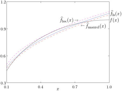
• Monomial approximation that minimizes maximum relative error Fig. 12 Relative error distributions for the three monomial approximations f loc , f ls , and f maxrel across the interval, with most errors under 3%, but maximum relative error exceeding 8%, also known as f maxrel (x).
• To find such vectors (and also the number k), the authors compute the SVD of the matrix [Y T 1].

9.1 Signomial programming

• Unfortunately some authors use the term 'generalized geometric program' to refer to a signomial program.
• The authors describe one general method for finding a local solution of an optimization problem that has the same form as a GP, but the objective and inequality constraint functions are not posynomials, and the equality constraint functions are not monomials.
• For the objective and each constraint function, the authors find the best local monomial approximation near the current guess x (k) , using the formula (40).
• The algorithm consists of repeating this step until convergence.
• It need not converge (but very often does), and can converge to a point that is not the global solution.

9.2 Mixed-integer geometric programming

• In a mixed-integer GP, the authors have a GP with the additional constraint that some of the variables lie in some discrete set, such as the integers: (46) where N denotes the set of natural numbers, i.e., positive integers.
• Then for each discrete variable that is within, say, 0.1 of an integer, the authors round it, and fix its value.
• The authors solve the relaxed GP, which gives us a lower bound on the optimal value of the MIGP, and they also use some heuristic (such as rounding) to find a locally optimal approximate solution.
• 10 Notes and references 10.1 Origins of geometric programming Geometric programming was introduced by Duffin, Peterson, and Zener in their (1967) book.

10.2 Algorithms and software

• In the early work by Duffin, Peterson, Zener, and Wilde, GPs were solved analytically via the dual problem (which is possible only for very small problems).
• These methods were based on solving a sequence of linear programs.
• Both packages include a simple interface to the MathWorks' MATLAB.
• Examples are CVX (Grant et al. 2005) , GGPLAB (Mutapcic et al. 2006) , and YALMIP (Löfberg 2003) , which have a simple interface that recognizes some GGPs, and automatically forms and solves the resulting GPs.

10.3 Applications

• Since its inception, GP has been closely associated with applications in engineering.
• In 1997, Hershenson, Boyd, and Lee applied GP to analog integrated circuit design (Hershenson et al. 2001) .

Figures

Fig. 1 Optimal trade-off curves of maximum volume V versus maximum floor area Aflr, for three values of maximum wall area Awall

Fig. 11 The solid curve is f (x)= √ 1 − (x − 1)2. f̂loc(x): best monomial approximation near x = 0.5. f̂ls(x): monomial approximation obtained via least-squares fitting to logarithmically transformed data. f̂maxrel(x): monomial approximation that minimizes maximum relative error

Fig. 4 Digital circuit with 7 gates

Fig. 10 The three functions given in (37), on a log-log plot

Fig. 5 Optimal trade-off curves of minimum delay Dmin versus maximum power Pmax, for three values of maximum area Amax

Fig. 8 Wire segment with length li and width wi (left) and its π model (right)

Fig. 9 RC tree model of the interconnect network in Fig. 7 using the π model

Fig. 2 A floor planning example with four rectangles A, B , C, and D

Fig. 13 Relative error distributions for max-monomial approximations, with three terms (̂h3), five terms (̂h5), and seven terms (̂h7 )

Table 1 Changes in maximum volume with changes in floor and wall area constraints. The first two columns give the change in the constraints. The third column gives the actual change in maximum volume, found by solving the GP with the new constraints, and the fourth column gives the change in maximum volume predicted by the optimal sensitivities

Fig. 15 Optimal trade-off curves of minimum delay Dmin versus maximum power Pmax, for the maximum area Amax = 100, with and without the constraint that the gate scale factors are integers

Fig. 6 Left. Two-bar truss. Right. Cross section of the bars

Fig. 3 Optimal trade-off curves of minimum bounding box area versus maximum aspect ratio αmax

Fig. 14 Relative error distributions for the posynomial approximations obtained via nonlinear least-squares fitting. ĥ3: 3-term posynomial fitting. ĥ5: 5-term posynomial fitting. ĥ7 : 7-term posynomial fitting

Full text

Optim Eng (2007) 8: 67–127
DOI 10.1007/s11081-007-9001-7
EDUCATIONAL SECTION
A tutorial on geometric programming
Stephen Boyd ·Seung-Jean Kim ·
Lieven Vandenberghe ·Arash Hassibi
Received: 17 March 2005 / Revised: 15 September 2005 /
Published online: 10 April 2007
© Springer Science+Business Media, LLC 2007
Abstract A geometric program (GP) is a type of mathematical optimization problem
characterized by objective and constraint functions that have a special form. Recently
developed solution methods can solve even large-scale GPs extremely efficiently and
reliably; at the same time a number of practical problems, particularly in circuit de-
sign, have been found to be equivalent to (or well approximated by) GPs. Putting
these two together, we get effective solutions for the practical problems. The basic
approach in GP modeling is to attempt to express a practical problem, such as an en-
gineering analysis or design problem, in GP format. In the best case, this formulation
is exact; when this is not possible, we settle for an approximate formulation. This
tutorial paper collects together in one place the basic background material needed
to do GP modeling. We start with the basic definitions and facts, and some methods
used to transform problems into GP format. We show how to recognize functions and
problems compatible with GP, and how to approximate functions or data in a form
compatible with GP (when this is possible). We give some simple and representative
examples, and also describe some common extensions of GP, along with methods for
solving (or approximately solving) them.
S. Boyd · S.-J. Kim (

)
Information Systems Laboratory, Department of Electrical Engineering, Stanford University,
Stanford, CA 94305, USA
e-mail: sjkim@stanford.edu
S. Boyd
e-mail: boyd@stanford.edu
L. Vandenberghe
Department of Electrical Engineering, University of California, Los Angeles, CA 90095, USA
e-mail: vandenbe@ucla.edu
A. Hassibi
Clear Shape Technologies, Inc., Sunnyvale, CA 94086, USA
e-mail: arash@clearshape.com

68 S. Boyd et al.
Keywords Convex optimization · Geometric programming ·
Generalized geometric programming · Interior-point methods
1 The GP modeling approach
A geometric program (GP) is a type of mathematical optimization problem charac-
terized by objective and constraint functions that have a special form. The importance
of GPs comes from two relatively recent developments:
• New solution methods can solve even large-scale GPs extremely efficiently and
reliably.
• A number of practical problems, particularly in electrical circuit design, have re-
cently been found to be equivalent to (or well approximated by) GPs.
Putting these two together, we get effective solutions for the practical problems. Nei-
ther of these developments is widely known, at least not yet. Nor is the story over:
Further improvements in GP solution methods will surely be developed, and, we be-
lieve, many more practical applications of GP will be discovered. Indeed, one of our
principal aims is to broaden knowledge and awareness of GP among potential users,
to help accelerate the hunt for new practical applications of GP.
The basic approach is to attempt to express a practical problem, such as an engi-
neering analysis or design problem, in GP format. In the best case, this formulation is
exact; when this isn’t possible, we settle for an approximate formulation. Formulating
a practical problem as a GP is called GP modeling. If we succeed at GP modeling,
we have an effective and reliable method for solving the practical problem.
We will see that GP modeling is not just a matter of using some software package
or trying out some algorithm; it involves some knowledge, as well as creativity, to be
done effectively. Moreover, success isn’t guaranteed: Many problems simply cannot
be represented, or even approximated, as GPs. But when we do succeed, the results
are very useful and impressive, since we can reliably solve even large-scale instances
of the practical problem.
It’s useful to compare GP modeling and modeling via general purpose nonlinear
optimization (also called nonlinear programming, or NLP). NLP modeling is rela-
tively easy, since the objective and constraint functions can be any nonlinear func-
tions. In contrast, GP modeling can be much trickier, since we are rather constrained
in the form the objective and constraint functions can take. Solving a GP is very easy;
but solving a general NLP is far trickier, and always involves some compromise (such
as accepting a local instead of a global solution). When we do GP modeling, we are
limiting the form of the objective and constraint functions. In return for accepting
this limitation, though, we get the benefit of extremely efficient and reliable solution
methods, that scale gracefully to large-scale problems.
A good analogy can be made with linear programming (LP). A linear program is
an optimization problem with an even stricter limitation on the form of the objective
and constraint functions (i.e., they must be linear). Despite what appears to be a very
restrictive form, LP modeling is widely used, in many practical fields, because LPs
can be solved with great reliability and efficiency. (This analogy is no accident—LPs
and GPs are both part of the larger class of convex optimization problems.)

A tutorial on geometric programming 69
This tutorial paper collects together in one place the basic background material
needed to do GP modeling. We start with the basic definitions and facts, and some
methods used to transform problems into GP format. We show how to recognize
functions and problems compatible with GP, and how to approximate functions or
data in a form compatible with GP (when this is possible). We give some simple and
representative examples, and also describe some common extensions of GP, along
with methods for solving (or approximately solving) them. This paper does not cover
the detailed theory of GPs (such as optimality conditions or duality) or algorithms
for solving GPs; our focus is on GP modeling.
This tutorial paper is organized as follows. In Sect. 2, we describe the basic form of
a GP and some simple extensions, and give a brief discussion of how GPs are solved.
We consider feasibility analysis, trade-off analysis, and sensitivity analysis for GPs
in Sect. 3, illustrated with simple numerical examples. In Sect. 4, we give two longer
examples to illustrate GP modeling, one from wireless communications, and the other
from semiconductor device engineering. We move on to generalized geometric pro-
gramming (GGP), a significant extension of GP, in Sect. 5, and give a number of ex-
amples from digital circuit design and mechanical engineering in Sect. 6. In Sect. 7,
we describe several more advanced techniques and extensions of GP modeling, and
in Sect. 8 we describe practical methods for fitting a function or some given data in a
form that is compatible with GP. In Sect. 9 we describe some extensions of GP that
result in problems that, unlike GP and GGP, are difficult to solve, as well as some
heuristic and nonheuristic methods that can be used to solve them. We conclude the
tutorial with notes and references in Sect. 10.
2 Basic geometric programming
2.1 Monomial and posynomial functions
Let x
1
,...,x
n
denote n real positive variables, and x = (x
1
,...,x
n
) a vector with
components x
i
. A real valued function f of x, with the form
f(x)=cx
a
1
1
x
a
2
2
···x
a
n
n
, (1)
where c>0 and a
i
∈R, is called a monomial function, or more informally, a mono-
mial (of the variables x
1
,...,x
n
). We refer to the constant c as the coefficient of the
monomial, and we refer to the constants a
1
,...,a
n
as the exponents of the monomial.
As an example, 2.3x
2
1
x
−0.15
2
is a monomial of the variables x
1
and x
2
, with coefficient
2.3 and x
2
-exponent −0.15.
Any positive constant is a monomial, as is any variable. Monomials are closed
under multiplication and division: if f and g are both monomials then so are fg
and f/g. (This includes scaling by any positive constant.) A monomial raised to any
power is also a monomial:
f(x)
γ
=(cx
a
1
1
x
a
2
2
···x
a
n
n
)
γ
=c
γ
x
γa
1
1
x
γa
2
2
···x
γa
n
n
.
The term ‘monomial’, as used here (in the context of geometric programming)
is similar to, but differs from the standard definition of ‘monomial’ used in algebra.

70 S. Boyd et al.
In algebra, a monomial has the form (1), but the exponents a
i
must be nonnegative
integers, and the coefficient c is one. Throughout this paper, ‘monomial’ will refer to
the definition given above, in which the coefficient can be any positive number, and
the exponents can be any real numbers, including negative and fractional.
A sum of one or more monomials, i.e., a function of the form
f(x)=
K

k=1
c
k
x
a
1k
1
x
a
2k
2
···x
a
nk
n
, (2)
where c
k
> 0, is called a posynomial function or, more simply, a posynomial (with
K terms, in the variables x
1
,...,x
n
). The term ‘posynomial’ is meant to suggest a
combination of ‘positive’ and ‘polynomial’.
Any monomial is also a posynomial. Posynomials are closed under addition, mul-
tiplication, and positive scaling. Posynomials can be divided by monomials (with the
result also a posynomial): If f is a posynomial and g is a monomial, then f/g is a
posynomial. If γ is a nonnegative integer and f is a posynomial, then f
γ
always
makes sense and is a posynomial (since it is the product of γ posynomials).
Let us give a few examples. Suppose x, y, and z are (positive) variables. The
functions (or expressions)
2x, 0.23, 2z

x/y, 3x
2
y
−.12
z
are monomials (hence, also posynomials). The functions
0.23 +x/y, 2(1 +xy)
3
, 2x +3y +2z
are posynomials but not monomials. The functions
−1.1, 2(1 +xy)
3.1
, 2x +3y −2z, x
2
+tan x
are not posynomials (and therefore, not monomials).
2.2 Standard form geometric program
A geometric program (GP) is an optimization problem of the form
minimize f
0
(x)
subject to f
i
(x) ≤1,i=1,...,m,
g
i
(x) =1,i=1,...,p,
(3)
where f
i
are posynomial functions, g
i
are monomials, and x
i
are the optimization
variables. (There is an implicit constraint that the variables are positive, i.e., x
i
> 0.)
We refer to the problem (3) as a geometric program in standard form, to distinguish
it from extensions we will describe later. In a standard form GP, the objective must
be posynomial (and it must be minimized); the equality constraints can only have the
form of a monomial equal to one, and the inequality constraints can only have the
form of a posynomial less than or equal to one.

A tutorial on geometric programming 71
As an example, consider the problem
minimize x
−1
y
−1/2
z
−1
+2.3xz +4xyz
subject to (1/3)x
−2
y
−2
+(4/3)y
1/2
z
−1
≤1,
x +2y +3z ≤1,
(1/2)xy =1,
with variables x, y and z. This is a GP in standard form, with n =3 variables, m =2
inequality constraints, and p =1 equality constraints.
We can switch the sign of any of the exponents in any monomial term in the
objective or constraint functions, and still have a GP. For example, we can change the
objective in the example above to x
−1
y
1/2
z
−1
+2.3xz
−1
+4xyz, and the resulting
problem is still a GP (since the objective is still a posynomial). But if we change
the sign of any of the coefficients, or change any of the additions to subtractions,
the resulting problem is not a GP. For example, if we replace the second inequality
constraint with x +2y −3z ≤1, the resulting problem is not a GP (since the left-hand
side is no longer a posynomial).
The term geometric program was introduced by Duffin, Peterson, and Zener in
their 1967 book on the topic (Duffin et al. 1967). It’s natural to guess that the name
comes from the many geometrical problems that can be formulated as GPs. But in
fact, the name comes from the geometric-arithmetic mean inequality, which played a
central role in the early analysis of GPs.
It is important to distinguish between geometric programming, which refers to
the family of optimization problems of the form (3), and geometric optimization,
which usually refers to optimization problems involving geometry. Unfortunately,
this nomenclature isn’t universal: a few authors use ‘geometric programming’ to
mean optimization problems involving geometry, and vice versa.
2.3 Simple extensions of GP
Several extensions are readily handled. If f is a posynomial and g is a monomial, then
the constraint f(x)≤g(x) can be handled by expressing it as f(x)/g(x)≤1 (since
f/g is posynomial). This includes as a special case a constraint of the form f(x)≤a,
where f is posynomial and a>0. In a similar way if g
1
and g
2
are both monomial
functions, then we can handle the equality constraint g
1
(x) =g
2
(x) by expressing it
as g
1
(x)/g
2
(x) = 1 (since g
1
/g
2
is monomial). We can maximize a nonzero mono-
mial objective function, by minimizing its inverse (which is also a monomial).
As an example, consider the problem
maximize x/y
subject to 2 ≤x ≤3,
x
2
+3y/z ≤
√
y,
x/y =z
2
,
(4)

Frequently asked questions

Q1. What contributions have the authors mentioned in the paper "A tutorial on geometric programming" ?

This tutorial paper collects together in one place the basic background material needed to do GP modeling. The authors show how to recognize functions and problems compatible with GP, and how to approximate functions or data in a form compatible with GP ( when this is possible ). The authors give some simple and representative examples, and also describe some common extensions of GP, along with methods for solving ( or approximately solving ) them. 

Q2. What is the main trick to solving a GP efficiently?

The main trick to solving a GP efficiently is to convert it to a nonlinear but convex optimization problem, i.e., a problem with convex objective and inequality constraint functions, and linear equality constraints. 

Q3. What is the way to fit a model to a monomial?

One useful extension of monomial fitting is to include a constant offset, i.e., to fit the data (x(i), f (i)) to a model of the formf (x) = b + cxa11 · · ·xann ,where b ≥ 0 is another model parameter. 

Q4. What are the posynomial functions of the wire segment widths wi?

The wire segment resistance and capacitance are both posynomial functions of the wire widths wi , which will be their design variables. 

Q5. What is the common method for finding the trade-off curve of the objective and one or?

Another common method for finding the trade-off curve (or surface) of the objective and one or more constraints is the weighted sum method. 

Q6. What is the constraint that the truss should be strong enough to carry the load?

The constraint that the truss should be strong enough to carry the load F1 means that the stress caused by the external force F1 must not exceed a given maximum value. 

Q7. What are the applications of geometric programming in other fields?

Applications of geometric programming in other fields include:• Chemical engineering (Clasen 1984; Salomone and Iribarren 1993; Salomone et al. 

Q8. How did the authors find the posynomial approximations for the same number?

The authors illustrate posynomial fitting using the same data points as those used in the max-monomial fitting example given in Sect. 8.4. The authors used a Gauss-Newton method to find K-term posynomial approximations, ĥK(x), for K = 3, 5, 7, which (locally, at least) minimize the sum of the squares of the relative errors. 

Q9. How do the authors find the optimal trade-off curve?

The optimal trade-off curve (or surface) can be found by solving the perturbed GP (12) for many values of the parameter (or parameters) to be varied. 

Q10. How can the authors handle a generalized posynomial with a negative coefficient?

This analysis suggests that the authors can handle composition of a generalized posynomial with any function whose series expansion has no negative coefficients, at least approximately, by truncating the series. 

Q11. What is the definition of a nonlinear least-squares problem?

This is a nonlinear least-squares problem, which can be solved (usually) using methods such as the Gauss-Newton method (Bertsekas 1999; Luenberger 1984; Nocedal and Wright 1999). 

Q12. What is the problem of finding a local monomial approximation of a?

8.2 Local monomial approximationThe authors consider the problem of finding a monomial approximation of a differentiable positive function f near a point x (with xi > 0). 

Q13. What is the method for the case with only one generalized posynomial equality?

The authors first describe the method for the case with only one generalized posynomial equality constraint (since it is readily generalizes to the case of multiple generalized posynomial equality constraints). 

Q14. what is the converse for generalized posynomials?

The interesting part here is the converse for generalized posynomials, i.e., the observation that if F can be approximated by a convex function, then f can be approximated by a generalized posynomial.