
All figures (10)
 Figure 5. Evolution of the EM (top panel) and the GW luminosity (bottom panel) integrated over 2-spheres located, respectively, at r = 20, 100, and 180M . Thick lines refer to the diffused emission, while thin ones to the emission from a polar cap of 5◦ semi-opening angle; the data refer to the spinning s6 binary and both the EM and the GW luminosities are computed including modes up to the = 8 multipole. Note that the gravitational-wave zone is already well defined at 100M , while the EM one is not even at 180M .
 Figure 1. Top row: orthogonality condition (left panel) and current-sheet condition (right panel) for a single spinning BH (dimensionless spin parameter a = J/M2 = 0.7), using different prescriptions for the current: fully discrete approach (light-blue solid line), driver1 plus discrete2 (red dotted line), driver1 plus continuum (dark-blue dashed line), driver1 plus driver2 (black long-dashed line). Bottom row: the same as in the top row, but for the equal-mass non-spinning binary BH system s0.
 Figure 4. Time evolution measured in hours before the merger of the EM luminosity at 100M when M = 108 M and B0 = 104 G. The thick lines refer to the total luminosity, while the thin ones to the luminosity in a polar cap of 5◦ semi-opening angle, measured using either expression (39) (red solid line), expression (40) (blue dotted line), or the flux using the Poynting vector in (41) (black dashed line). The left panel refers to the binary of non-spinning BHs (i.e., s0), while the right one to the binary with spinning BHs (i.e., s6). Note that in this latter case a certain eccentricity is detectable in the EM luminosity, although it is much smaller in the GW luminosity.
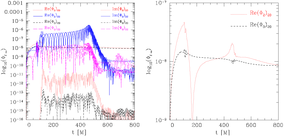 Figure 3. Left panel: evolution of the real (thick lines) and imaginary (thin lines) parts of the = 2,m = 0 and = 2,m = 2 modes of Φ2 and Φ0, extracted at 100M for the non-spinning binary s0. Right panel: the same as in the left panel but with a scale appropriate to highlight the evolution of Re(Φ2)20 (red dotted line) and of Re(Φ0)20 (black dashed line). Both are almost constant in time and comparable, but not identical.
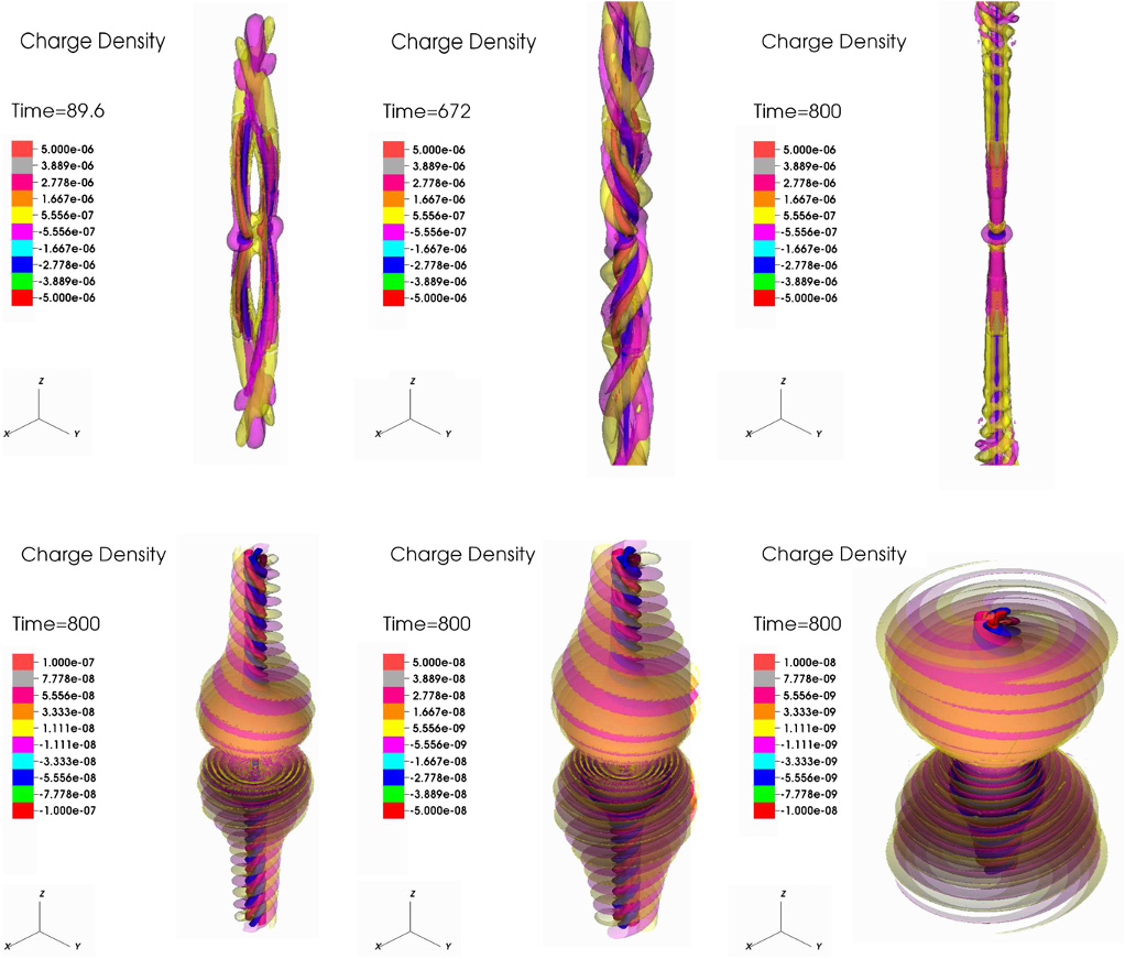 Figure 8. Top row: large-scale three-dimensional distribution of the charge density for the s6 binary in the early inspiral phase at t = 89M (left panel), at the merger t = 672M (middle panel), and at ringdown t = 800M (right panel). In these panels only the largest values of the charge density are shown. Bottom row: three-dimensional distribution of the charge density at ringdown only, t = 800M . Starting from the left, the panels show smaller and smaller values of the charge density, revealing a much more extended conical-shaped structure with a double-helical distribution of opposite charges. Clearly, charge-density distribution is far more complex than what would be deduced from the top panels only.
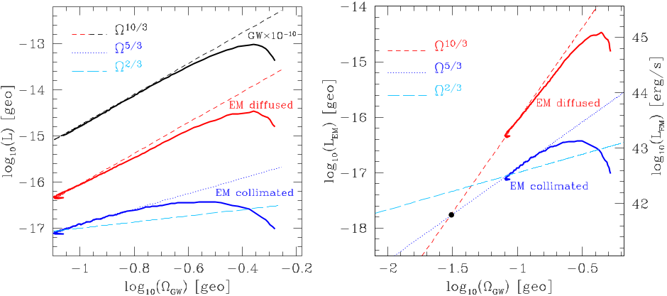 Figure 6. Left panel: frequency scaling for the non-spinning binary s0 of the GW luminosity rescaled of a factor 10−10 (black solid line), of the diffused EM luminosity (red solid line), and of the collimated EM luminosity computed in a polar cap with a semi-opening angle of 5◦ (blue solid line). Note that the diffused EM luminosity has a behavior which is compatible with Ω10/3−8/3 as does as the GW luminosity. The collimated EM luminosity, on the other hand, has a scaling compatible with Ω5/3−6/3. Right panel: the same as in the left panel but reporting only the GW emission and extrapolating back in the past to determine when the collimated and the diffused emissions are comparable. For a binary with 108 M this happens ∼21 days before merger.
 Figure 7. Small-scale two-dimensional distribution of the charge density for a s6 binary in the early inspiral phase at t = 89M (left column), at merger t = 672M (middle column), and at ringdown t = 800M (right column). The top panels show the charge density in the (x, y) plane, while the bottom ones in the (x, z) plane. Visualizations artifacts appear as thin stripes at the boundaries between refinement levels; the data in those stripes are of course regular.
 Figure 2. Comparison of the electric currents for a single spinning BH with dimensionless spin parameter a = J/M2 = 0.7 on the plane (x, y, z = 1.92M) (top row) and on the plane (x, y = 0, z) (bottom row). All panels refer to the same time t = 102M , when the solution has reached a stationary state. The currents are computed either through the fully discrete approach of discrete1–discrete2 (left column) or through our continuous driver1–driver2 approach (right column). While both solutions satisfy the FF condition, it is clear that the use of the drivers provides also an accurate solution.
 Table 1 Explicit IMEX-SSP3(4,3,3) L-stable Scheme
 Table 2 Implicit IMEX-SSP3(4,3,3) L-stable Scheme


