
All figures (55)

Fig. 72 L/D vs. angle of attack: monoplane vs. biplane: In order to make a final choice about which wing configuration should be used for the Small UAV under design, an equivalent monoplane was considered and modelled with the software AVL, and then compared to the nonplanar configuration under study. This figure shows a comparison in the L/D ratio vs. angle of attack between the two configurations. 
Fig. 41: gust diagram for a Small UAV. For each of the characteristic speeds, stall, cruise and dive speed, the load factor was calculated. It can be noticed that the highest load factor is reached for the cruise speed and is 3.92. 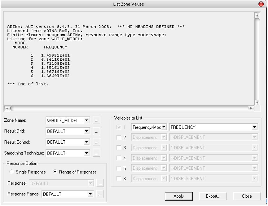
Fig. 55 Adina: natural frequencies: ADINA can also determine the first few natural frequencies and modes for the structure under study. A list of the natural frequencies can be displayed as shown in this figure. The first mode happens at 14.9 Hz, the second at 63.6 Hz and the third at 87.11 Hz. 
Fig. 60 Stress variation with gap and stagger: This figure shows a plot where the change in max 
Fig. 15 Constraint diagram: This figure shows the constraint diagram obtained plotting the constraint equations. This graph is very useful because each point of the design space in grey, represents a possible aircraft design for the class of aircraft and for the profile mission in consideration, based on physics alone 
Fig 12 Joined wing configuration: This figure represents a Joined wing configuration. The shape of a joined wing configuration is obtained by attaching the forward wing low on the fuselage, then sweeping backward and upward while tapering it to the tip. The aft wing is attached high on the vertical fin. ![Fig. 4 Gross mass of flying object vs Reynolds Number (partly reproduced from [6]): The graph shows the gross mass of small air vehicles and other flying objects vs chord Reynolds Number The Reynolds Number of Small Uavs has a similar order of magnitude as many birds as well as similar weight which may imply also similar aerodynamic behaviour.](/figures/fig-4-gross-mass-of-flying-object-vs-reynolds-number-partly-4ppb9psr.png)
Fig. 4 Gross mass of flying object vs Reynolds Number (partly reproduced from [6]): The graph shows the gross mass of small air vehicles and other flying objects vs chord Reynolds Number The Reynolds Number of Small Uavs has a similar order of magnitude as many birds as well as similar weight which may imply also similar aerodynamic behaviour. 
Fig. 10 illustrates the reduction of drag against lift coefficient for various 
Table 1 UAV previous successful designs: This table reports per each row the primary conceptual design characteristics for 7 different successful UAV designs. This table is very important to start to have a feeling for the order of magnitude of these characteristics for this class of aircraft. 
Fig. 16 Constraint diagram and previous designs: This figure shows the constraint diagram for the class of aircraft under consideration obtained plotting the constraint equations and the design points of previous small UAV. It can be noticed that bungee cord launched UAVs have different assumptions, like different stall velocity and therefore the points which represent these configuration in this graph fall outside the design space. 
Table 11 displacement and maximum effective stresses for a biplane: Using the software ADINA, the displacement and maximum effective stresses were calculated for eight models of standard biplane not joined at the tips with flow guides.. It can be noticed that the displacement and the Max Effective Stress for the biplane configuration remain the same for all the configurations. 
Fig. 61 Stress variation with stagger and gap: This figure shows a plot where the change in max effective stress with variation in the stagger while holding gap constant is reported for the standard biplane and for the configuration under study with a 0.5 and 1 gap. Increasing the gap the Displacement and the Maximum Effective stress of the biplane is constant. 
Fig. 56 Adina: mode shape: This figure displays the first mode shape of model # 1 with 0 stagger and 1c gap as an example. In this case it represents the first bending mode shape. At higher frequency there is also the first torsion shape mode. 
Table 10 displacement and maximum effective stress: Using the software ADINA, the displacement and maximum effective stresses were calculated for each configuration. It can be noticed that the configuration with 0.5 Gap and 0 Stagger has the smallest displacement and the model with 1 gap and 0 stagger has the smallest max effective stress. 
Fig. 42: example of wing box structure. Several elements can be noticed: 3 carbon fibre spar caps BB’, DD’, EE’, 1 spar DD’EE’ in carbon fibre, Foam core, Fibreglass skin. 
Table 8: properties of foam and balsa: The foam core carbon fibre composites have superior strength to weight ratios compared to balsa ribbed wings that utilize a carbon fibre tube spar, due to failure of the balsa ribs at lower loading, especially when normalized by the structural weight of each type of wing. 
Fig. 10 illustrates the reduction of drag against lift coefficient for various 
Fig. 71 Cl vs. angle of attack: monoplane vs biplane: In order to make a final choice about which wing configuration should be used for the Small UAV under design, an equivalent monoplane was considered and modelled with the software AVL, and then compared to the nonplanar configuration under study. This figure shows a comparison in the lift slope between the two configurations. ![Fig. 38 level of blur vs. velocity: The loiter speed is a variable controlled by the sensor payload because images become blurry at fast speeds. The graph shows for a wide variety of micro video cameras on market today, the maximum speed allowable before images become blurry (reproduced from [30]).](/figures/fig-38-level-of-blur-vs-velocity-the-loiter-speed-is-a-3rz432a2.png)
Fig. 38 level of blur vs. velocity: The loiter speed is a variable controlled by the sensor payload because images become blurry at fast speeds. The graph shows for a wide variety of micro video cameras on market today, the maximum speed allowable before images become blurry (reproduced from [30]). 
Fig. 63 Adina: Effective stress distribution of an equivalent monoplane: This figure represents in detail the Effective Stress distribution of an equivalent monoplane as obtained from the software ADINA when the wing undergoes to an elliptical lift distribution as calculated in the previous sections. The highest stress is located at the wing root. 
Fig. 69 Experimental results L/D vs angle of attack for different gap configurations: This 
Fig. 44 Elliptical distribution vs. constant-linear lift distribution: This graph shows a comparison between the Elliptical distribution and the constant-linear distribution of the lift along the semi span. The constant linear distribution, constant from the root to the 2/3 of the semi span and then linear from the 2/3 of the span to the tip of the wing, is introduced in order to simplify the calculations. ![Fig. 8 Stagger (reproduced by [8]): The stagger of a Biplane is one of the main geometrical characteristics of the biplane configuration. It is the relative longitudinal position of the wings on a biplane. Positive Stagger is when the upper wing's leading edge is in advance of that of the lower wing and vice versa for Negative Staggerlower wing [eg: Waco YKS], and vice versa for Negative Stagger](/figures/fig-8-stagger-reproduced-by-8-the-stagger-of-a-biplane-is-1h3b15og.png)
Fig. 8 Stagger (reproduced by [8]): The stagger of a Biplane is one of the main geometrical characteristics of the biplane configuration. It is the relative longitudinal position of the wings on a biplane. Positive Stagger is when the upper wing's leading edge is in advance of that of the lower wing and vice versa for Negative Staggerlower wing [eg: Waco YKS], and vice versa for Negative Stagger 
Table 2 Historical value: Historical values of Payload Weight Fractions. From this Table, Orbiter and Puma have the highest Payload fraction which is a predictable result: Pointer is an old UAV and at that time the payload was heavier than the modern miniaturized cameras, Orbiter is a bungee launched aircraft and therefore has a higher stall speed and therefore can carry a higher payload keeping constant all the other parameters. ![Fig. 1 (reproduced from [5]): The U.S. Unmanned System Roadmap. US Unmanned System Roadmap 2007-2032 predicts a general development and employment of unmanned systems in the future. In particular, the figure shows an increase in the number of UAS for Oceanography digital mapping and suppression of enemy air defences by the Air Force and an increase in UAS for communications, navigation network node, electronic warfare, psychological operations by the Navy.](/figures/fig-1-reproduced-from-5-the-u-s-unmanned-system-roadmap-us-illzg8lp.png)
Fig. 1 (reproduced from [5]): The U.S. Unmanned System Roadmap. US Unmanned System Roadmap 2007-2032 predicts a general development and employment of unmanned systems in the future. In particular, the figure shows an increase in the number of UAS for Oceanography digital mapping and suppression of enemy air defences by the Air Force and an increase in UAS for communications, navigation network node, electronic warfare, psychological operations by the Navy. 
Fig. 18 shows the variation in the design space with the variation in TOd . 
Fig. 57 Adina: configuration with the smallest displacement: from Table 10 it can be seen that the configuration with the smallest displacement is model #2 with 0.5C gap and 0 stagger, it’s displacement distribution is reported in this figure. 
Fig. 58 Adina: configuration with largest displacement: from Table 10 that the model with the largest displacement and largest effective stress at the root is model #8 with 1c gap and 1.5c stagger. Its displacement distribution is reported in this figure. 
Fig. 6 wing geometry and trailing vortex wake: Specifying the geometry of the trailing vortex wake and solving for the circulation distribution with minimum drag, Kroo obtained as a result that the boxplane represents the minimum solution. All the non planar geometries he took in consideration have same projected span and lift. 
Table 5 Weight builds up: the different parts of the aircraft are reported with their weight and then added together. Four main different components have been individuated: The motor, the battery, the avionics and payload and the airframe. The total weight is 3091.6 g. ![Fig. 32 Weight breakdown: This graph represents the component weight breakdown of the aircraft. The main weight is estimated to come from the airframe then the second biggest weight come from the battery. A battery weight in the neighbourhood of at least 25% of the gross weight or more should be considered [4.4.4.]; below 25%, the endurance potential declines more and more deeply.](/figures/fig-32-weight-breakdown-this-graph-represents-the-component-33e1f96s.png)
Fig. 32 Weight breakdown: This graph represents the component weight breakdown of the aircraft. The main weight is estimated to come from the airframe then the second biggest weight come from the battery. A battery weight in the neighbourhood of at least 25% of the gross weight or more should be considered [4.4.4.]; below 25%, the endurance potential declines more and more deeply. 
Fig. 52 Adina: mesh density creation: After approximating the behaviour of the structure with Shell elements, a uniform mesh density was created with four nodes per element. This figure shows the graphic window of ADINA for model 1 after the mesh. 
Table 12 Decision analysis: In order to make a final choice and proceed with the following design steps, a decision analysis was performed. % Criteria were chosen and 3 configuration analyzed. The criteria reflects the specifications expressed in the requirements of Chapter III. The most important criteria selected was the weight. The final score shows a slightly greater score for the joined at the tips configuration. 
Table 3 Selected battery combination: The table shows the selected battery combination: 5 batteries in series and 4 in parallel. The capacity of 8000 mAh meets the endurance requirements and the weight equals to the 26% of the gross weight is in agreement with section 4.4.4.1 
Fig. 22 Comparative UAVs: Photos of comparative small UAVs: these photos can help to have a visual understanding of the class of aircraft under consideration. From the top left to the bottom the pictures represent: Pointer, Raven, Puma, Dragon Eye, Desert Hawk, Orbiter and Metu Guventurk. From this pictures it can be also noticed the different layouts used for the different small UAV. 
Fig. 64 Adina: Stress distribution of an equivalent monoplane with same span of the nonplanar configuration: This figure represents in detail the Effective Stress distribution of an equivalent monoplane with same span of the nonplanar configuration under consideration as obtained from the software ADINA when the wing undergoes to an elliptical lift distribution as calculated in the previous sections. The highest stress is located at the wing root. ![Fig. 7 Gap (reproduced by [8]): The gap of a Biplane is one of the main geometrical characteristics of the biplane configuration. It is the distance between the planes of the chords measured along a line perpendicular to the chords](/figures/fig-7-gap-reproduced-by-8-the-gap-of-a-biplane-is-one-of-the-3ma2gw5j.png)
Fig. 7 Gap (reproduced by [8]): The gap of a Biplane is one of the main geometrical characteristics of the biplane configuration. It is the distance between the planes of the chords measured along a line perpendicular to the chords 
Fig. 13 Houck configuration: This figure represents the Houck Configuration which is the configuration this study inspires to. This concept combines an upper and lower wing joined at the tips with flow guides with the intent of significantly reducing vortex losses caused by span wise fluid flow and induced drag. 
Fig. 40: Scheme of vertical gusts: a small UAV reacts easily to the force of the wind, therefore the loads associated with vertical gusts must also be evaluated over the range of speeds. UG is the speed of the gusts, V represents the speed of the airplane and α∆ represents the change in angle of attack due to the gusts. 
Table 6 Design parameters: In this table the main characteristics of the aircraft after the change in weight are reported. Once the first iteration has been completed it is easy to insert just the new values and complete a second more refined iteration. ![Fig 11 Gage’s complexity evolutionary algorithm: In 1994 Gage [13] produced a complexity evolutionary algorithm, which was allowed to build wings in many individual elements with arbitrary dihedral and optional twist. The system when it evolves discovers winglets and then adds a horizontal extension to the winglets, forming a C like shape as shown in the figure.](/figures/fig-11-gages-complexity-evolutionary-algorithm-in-1994-gage-10e5x553.png)
Fig 11 Gage’s complexity evolutionary algorithm: In 1994 Gage [13] produced a complexity evolutionary algorithm, which was allowed to build wings in many individual elements with arbitrary dihedral and optional twist. The system when it evolves discovers winglets and then adds a horizontal extension to the winglets, forming a C like shape as shown in the figure. ![Fig. 5 Relative vortex vs Overall Height/Span (partly reproduced from [6]): From the results obtained by Kroo [6] a ring wing has half of the vortex drag of a monoplane of the same span and lift, and the boxplane has the lowest drag for a given span and height. From an aerodynamic point of view it means that keeping fixed the span considerable savings in induced drag can be achieved if large vertical extents are permitted. Of course structural considerations must be considered too.](/figures/fig-5-relative-vortex-vs-overall-height-span-partly-1o6qov51.png)
Fig. 5 Relative vortex vs Overall Height/Span (partly reproduced from [6]): From the results obtained by Kroo [6] a ring wing has half of the vortex drag of a monoplane of the same span and lift, and the boxplane has the lowest drag for a given span and height. From an aerodynamic point of view it means that keeping fixed the span considerable savings in induced drag can be achieved if large vertical extents are permitted. Of course structural considerations must be considered too. 
Fig. 53 Adina: examination of the solution: After saving the model and running it in ADINA, the PostProcessing function must be opened in order to examine the solution. The displacements can easily be visualized through a band plot. In this figure the band plot for model #1 with 1 gap and 0 stagger is reported, which shows the displacement distribution. As could be predicted, the major displacement is on the wing tip. 
Fig. 45: Lift and drag distribution along the semi span. The lift is constant from the root to the 2/3 of the semi span and then linear from the 2/3 of the span to the tip of the wing. The drag is considered as a first approximation, constant along the span. ![Fig. 3 UAVs Classification (reproduced from [5]): UAVs can be classified in different ways. JUAS COE gives a classification on the basis of airspeed, weight and operating altitude. This thesis focuses on level 1 UAS. The weight ranges form 2 to 20 lbs and the operating altitude is less than 3,000 feet.](/figures/fig-3-uavs-classification-reproduced-from-5-uavs-can-be-2anvualu.png)
Fig. 3 UAVs Classification (reproduced from [5]): UAVs can be classified in different ways. JUAS COE gives a classification on the basis of airspeed, weight and operating altitude. This thesis focuses on level 1 UAS. The weight ranges form 2 to 20 lbs and the operating altitude is less than 3,000 feet. 
Fig. 2: UAVS Classification. UAVs can be classified in different ways. This figure represents a UAV classification with respect to weight and wingspan. In this case there are 4 different groups: micro, small, medium and large. This thesis focuses on small UAVs. 
Fig. 27 Types of electric motors: There are 3 basic types of electric motors suitable for Small UAV applications and they are shown in this picture. On the left there is a traditional brushed motor. In the middle there is an inner brushless motor and on the right there is an outrunner brushless motor. 
Fig. 59 Adina stress distribution of configuration with largest displacement and effective stress: from Table 10 that the model with the largest displacement and largest effective stress at the root is model #8 with 1c gap and 1.5c stagger. Its stress distribution is reported in this figure. 
Table 4 Vertical and horizontal tail specifications: This table shows the surfaces of the vertical and horizontal empennage. The A.R, chord and Span are also reported. 
Fig 14 Mission profile of a Small UAVs: Mission profile of a Small UAVs is composed of 6 different steps: After the take off, the airplane climb to the target altitude (ascent); after reaching this altitude there is cruise segment necessary to reach the mission target, then a phase of loitering around the target, finally a cruise to come back to the launching site, a descent and a landing, with or without a parachute. 
Fig. 70 AVL equivalent monoplane geometry: In order to make a final choice about which wing configuration should be used for the Small UAV under design, an equivalent monoplane was considered and modelled with the software AVL, and then compared to the nonplanar configuration under study. This figure shows the displayed image on the software AVL after all the geometrical inputs have been inserted in the code. ![Fig. 66 Gap vs lift reproduced from [#]:The gap, from the results of AVL has a big impact on the lift coefficient. Increasing the gap between the two lifting surfaces of a biplane will result in an increase in the total lift coefficient. A greater rate of increase in lift coefficient as a function of increasing gap is observed until the gap reaches approximately 1 chord length distance.](/figures/fig-66-gap-vs-lift-reproduced-from-the-gap-from-the-results-7o2wa5xb.png)
Fig. 66 Gap vs lift reproduced from [#]:The gap, from the results of AVL has a big impact on the lift coefficient. Increasing the gap between the two lifting surfaces of a biplane will result in an increase in the total lift coefficient. A greater rate of increase in lift coefficient as a function of increasing gap is observed until the gap reaches approximately 1 chord length distance. 
Fig. 33 and 34. The configuration described in Fig. 33 and the configurations described in Fig. 35 are very similar. The main difference is the use of endplates. In the next chapter it will be analyzed from a structural and aerodynamic point of view if using the configuration of Fig. 33 can bring any benefits with respect to the standard monoplane (Fig. 34) or with respect to the standard biplane (Fig. 35) ![Table 9 Physical characteristics of the models: this table represents the physical characteristics of the eight wing configurations that have been tested in the Low Speed Wind Tunnel (LSWT) [18] of the University of Dayton. The Aspect Ratio was calculated as 2b/c, the material used was stainless steel.](/figures/table-9-physical-characteristics-of-the-models-this-table-m5lzbzwu.png)
Table 9 Physical characteristics of the models: this table represents the physical characteristics of the eight wing configurations that have been tested in the Low Speed Wind Tunnel (LSWT) [18] of the University of Dayton. The Aspect Ratio was calculated as 2b/c, the material used was stainless steel. 
Table 7: UD for three characteristic conditions: gust, cruise and dive. Using these estimated speed it is possible to create the gust diagram reported in Fig. 37


![Fig. 4 Gross mass of flying object vs Reynolds Number (partly reproduced from [6]): The graph shows the gross mass of small air vehicles and other flying objects vs chord Reynolds Number The Reynolds Number of Small Uavs has a similar order of magnitude as many birds as well as similar weight which may imply also similar aerodynamic behaviour.](/figures/fig-4-gross-mass-of-flying-object-vs-reynolds-number-partly-4ppb9psr.webp)


![Fig. 38 level of blur vs. velocity: The loiter speed is a variable controlled by the sensor payload because images become blurry at fast speeds. The graph shows for a wide variety of micro video cameras on market today, the maximum speed allowable before images become blurry (reproduced from [30]).](/figures/fig-38-level-of-blur-vs-velocity-the-loiter-speed-is-a-3rz432a2.webp)


![Fig. 8 Stagger (reproduced by [8]): The stagger of a Biplane is one of the main geometrical characteristics of the biplane configuration. It is the relative longitudinal position of the wings on a biplane. Positive Stagger is when the upper wing's leading edge is in advance of that of the lower wing and vice versa for Negative Staggerlower wing [eg: Waco YKS], and vice versa for Negative Stagger](/figures/fig-8-stagger-reproduced-by-8-the-stagger-of-a-biplane-is-1h3b15og.webp)

![Fig. 1 (reproduced from [5]): The U.S. Unmanned System Roadmap. US Unmanned System Roadmap 2007-2032 predicts a general development and employment of unmanned systems in the future. In particular, the figure shows an increase in the number of UAS for Oceanography digital mapping and suppression of enemy air defences by the Air Force and an increase in UAS for communications, navigation network node, electronic warfare, psychological operations by the Navy.](/figures/fig-1-reproduced-from-5-the-u-s-unmanned-system-roadmap-us-illzg8lp.webp)


![Fig. 32 Weight breakdown: This graph represents the component weight breakdown of the aircraft. The main weight is estimated to come from the airframe then the second biggest weight come from the battery. A battery weight in the neighbourhood of at least 25% of the gross weight or more should be considered [4.4.4.]; below 25%, the endurance potential declines more and more deeply.](/figures/fig-32-weight-breakdown-this-graph-represents-the-component-33e1f96s.webp)


![Fig. 7 Gap (reproduced by [8]): The gap of a Biplane is one of the main geometrical characteristics of the biplane configuration. It is the distance between the planes of the chords measured along a line perpendicular to the chords](/figures/fig-7-gap-reproduced-by-8-the-gap-of-a-biplane-is-one-of-the-3ma2gw5j.webp)


![Fig 11 Gage’s complexity evolutionary algorithm: In 1994 Gage [13] produced a complexity evolutionary algorithm, which was allowed to build wings in many individual elements with arbitrary dihedral and optional twist. The system when it evolves discovers winglets and then adds a horizontal extension to the winglets, forming a C like shape as shown in the figure.](/figures/fig-11-gages-complexity-evolutionary-algorithm-in-1994-gage-10e5x553.webp)
![Fig. 5 Relative vortex vs Overall Height/Span (partly reproduced from [6]): From the results obtained by Kroo [6] a ring wing has half of the vortex drag of a monoplane of the same span and lift, and the boxplane has the lowest drag for a given span and height. From an aerodynamic point of view it means that keeping fixed the span considerable savings in induced drag can be achieved if large vertical extents are permitted. Of course structural considerations must be considered too.](/figures/fig-5-relative-vortex-vs-overall-height-span-partly-1o6qov51.webp)


![Fig. 3 UAVs Classification (reproduced from [5]): UAVs can be classified in different ways. JUAS COE gives a classification on the basis of airspeed, weight and operating altitude. This thesis focuses on level 1 UAS. The weight ranges form 2 to 20 lbs and the operating altitude is less than 3,000 feet.](/figures/fig-3-uavs-classification-reproduced-from-5-uavs-can-be-2anvualu.webp)


![Fig. 66 Gap vs lift reproduced from [#]:The gap, from the results of AVL has a big impact on the lift coefficient. Increasing the gap between the two lifting surfaces of a biplane will result in an increase in the total lift coefficient. A greater rate of increase in lift coefficient as a function of increasing gap is observed until the gap reaches approximately 1 chord length distance.](/figures/fig-66-gap-vs-lift-reproduced-from-the-gap-from-the-results-7o2wa5xb.webp)

![Table 9 Physical characteristics of the models: this table represents the physical characteristics of the eight wing configurations that have been tested in the Low Speed Wind Tunnel (LSWT) [18] of the University of Dayton. The Aspect Ratio was calculated as 2b/c, the material used was stainless steel.](/figures/table-9-physical-characteristics-of-the-models-this-table-m5lzbzwu.webp)

05 Jan 2009-