scispace - formally typeset
Search or ask a question
Journal ArticleDOI

Bayesian Estimation Supersedes the t Test

01 May 2013-Journal of Experimental Psychology: General (American Psychological Association)-Vol. 142, Iss: 2, pp 573-603
TL;DR: Bayesian estimation for 2 groups provides complete distributions of credible values for the effect size, group means and their difference, standard deviations and their Difference, and the normality of the data.
Abstract: Bayesian estimation for 2 groups provides complete distributions of credible values for the effect size, group means and their difference, standard deviations and their difference, and the normality of the data. The method handles outliers. The decision rule can accept the null value (unlike traditional t tests) when certainty in the estimate is high (unlike Bayesian model comparison using Bayes factors). The method also yields precise estimates of statistical power for various research goals. The software and programs are free and run on Macintosh, Windows, and Linux platforms.

Summary (2 min read)

1 Introduction

  • The BEST package provides a Bayesian alternative to a t test, providing much richer information about the samples and the difference in means than a simple p value.
  • Bayesian estimation for two groups provides complete distributions of credible values for the effect size, group means and their difference, standard deviations and their difference, and the normality of the data.
  • For a single group, distributions for the mean, standard deviation and normality are provided.
  • The decision rule can accept the null value (unlike traditional t tests) when certainty in the estimate is high (unlike Bayesian model comparison using Bayes factors).
  • The package also provides methods to estimate statistical power for various research goals.

2 The Model

  • To accommodate outliers the authors describe the data with a distribution that has fatter tails than the normal distribution, namely the t distribution.
  • (Note that the authors are using this as a convenient description of the data, not as a sampling distribution from which p values are derived.).
  • The data (y) are assumed to be independent and identically distributed (i.i.d.) draws from a t distribution with different mean (µ) and standard deviation (σ) for each population, and with a common normality parameter (ν), as indicated in the lower portion of Figure 1.
  • The default priors, with priors = NULL, are minimally informative: normal priors with large standard deviation for (µ), broad uniform priors for (σ), and a shifted-exponential prior for (ν), as described by Kruschke (2013).
  • These priors are indicated in the upper portion of Figure 1.

3 Preparing to run BEST

  • BEST uses the JAGS package (Plummer, 2003) to produce samples from the posterior distribution of each parameter of interest.
  • You will need to download JAGS from http://sourceforge.
  • Net/projects/mcmc-jags/ and install it before running BEST.
  • BEST also requires the packages rjags and coda, which should normally be installed at the same time as package BEST if you use the install.
  • Once installed, the authors need to load the BEST package at the start of each R session, which will also load rjags and coda and link to JAGS: > library(BEST).

4.2 Running the model

  • The authors run BESTmcmc and save the result in BESTout.
  • The authors do not use parallel processing here, but if your machine has at least 4 cores, parallel processing cuts the time by 50%.

4.3 Basic inferences

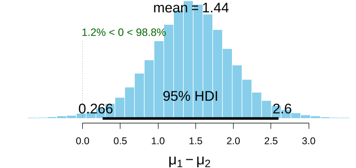
  • Also shown is the mean of the posterior probability, which is an appropriate point estimate of the true difference in means, the 95% Highest Density Interval (HDI), and the posterior probability that the difference is greater than zero.
  • An increase reaction time of 1 unit may indicate that users of the drug should not drive or operate equipment.
  • More interesting is the probability that the difference may be too small to matter.
  • But if most of the probability mass (say, 95%) lay within the ROPE, the authors would accept the null value for practical purposes.

4.4 Checking convergence and fit

  • The output from BESTmcmc has class BEST, which has a print method: > class [1].
  • 'Rhat' is the potential scale reduction factor (at convergence, Rhat=1).
  • Increase the burnInSteps argument to BESTmcmc if any of the Rhats are too big.
  • Values of n.eff around 10,000 are needed for stable estimates of 95% credible intervals.
  • The function plotAll puts histograms of all the posterior distributions and the posterior predictive plots onto a single page . > plotAll.

4.5 Working with individual parameters

  • Objects of class BEST contain long vectors of simulated draws from the posterior distribution of each of the parameters in the model.
  • You may wish to look at the ratio of the variances rather than the difference in the standard deviations.
  • You can calculate a vector of draws from the posterior distribution, calculate summary statistics, and plot the distribution with plotPost : > <- BESTout$sigma1^2 / BESTout$sigma2^2 > median [1].

5 An example with a single group

  • Applying BEST to a single sample, or for differences in paired observations, works in much the same way as the two-sample method and uses the same function calls.
  • To run the model, simply use BESTmcmc with only one vector of observations.
  • Standard deviation, the normality parameter and effect size can be plotted individually, or on a single page with plotAll . > plotAll(BESTout1g).

6 What next?

  • The package includes functions to estimate the power of experimental designs: see the help pages for BESTpower and makeData for details on implementation and Kruschke (2013) for background.
  • If you want to know how the functions in the BEST package work, you can download the R source code from CRAN or from GitHub https://github.com/mikemeredith/BEST.
  • For a practical introduction see Kruschke (2015).

7 References

  • A tutorial with R, JAGS and Stan, also known as Doing Bayesian data analysis.
  • In 3rd International Workshop on Distributed Statistical Computing (DSC 2003).

Did you find this useful? Give us your feedback

Content maybe subject to copyright    Report

Bayesian Estimation Supersedes the t-Test
Mike Meredith and John Kruschke
October 13, 2021
1 Introduction
The BEST package provides a Bayesian alternative to a t test, providing much richer information
about the samples and the difference in means than a simple p value.
Bayesian estimation for two groups provides complete distributions of credible values for the
effect size, group means and their difference, standard deviations and their difference, and the
normality of the data. For a single group, distributions for the mean, standard deviation and
normality are provided. The method handles outliers.
The decision rule can accept the null value (unlike traditional t tests) when certainty in the
estimate is high (unlike Bayesian model comparison using Bayes factors).
The package also provides methods to estimate statistical power for various research goals.
2 The Model
To accommodate outliers we describe the data with a distribution that has fatter tails than the
normal distribution, namely the t distribution. (Note that we are using this as a convenient
description of the data, not as a sampling distribution from which p values are derived.) The
relative height of the tails of the t distribution is governed by the shape parameter ν: when ν
is small, the distribution has heavy tails, and when it is large (e.g., 100), it is nearly normal.
Here we refer to ν as the normality parameter.
The data (y) are assumed to be independent and identically distributed (i.i.d.) draws from
a t distribution with different mean (µ) and standard deviation (σ) for each population, and
with a common normality parameter (ν), as indicated in the lower portion of Figure 1.
The default priors, with priors = NULL, are minimally informative: normal priors with
large standard deviation for (µ), broad uniform priors for (σ), and a shifted-exponential prior
for (ν), as described by Kruschke (2013). You can specify your own priors by providing a
list: population means (µ) have separate normal priors, with mean muM and standard deviation
muSD; population standard deviations (σ) have separate gamma priors, with mode sigmaMode
and standard deviation sigmaSD; the normality parameter (ν) has a gamma prior with mean
nuMean and standard deviation nuSD. These priors are indicated in the upper portion of Figure 1.
For a general discussion see chapters 11 and 12 of Kruschke (2015).
1

Figure 1: Hierarchical diagram of the descriptive model for robust Bayesian estimation.
3 Preparing to run BEST
BEST uses the JAGS package (Plummer, 2003) to produce samples from the posterior distribu-
tion of each parameter of interest. You will need to download JAGS from http://sourceforge.
net/projects/mcmc-jags/ and install it before running BEST.
BEST also requires the packages rjags and coda, which should normally be installed at the
same time as package BEST if you use the install.packages function in R.
Once installed, we need to load the BEST package at the start of each R session, which will
also load rjags and coda and link to JAGS:
> library(BEST)
4 An example with two groups
4.1 Some example data
We will use hypothetical data for reaction times for two groups (N
1
= N
2
= 6), Group 1
consumes a drug which may increase reaction times while Group 2 is a control group that
consumes a placebo.
> y1 <- c(5.77, 5.33, 4.59, 4.33, 3.66, 4.48)
> y2 <- c(3.88, 3.55, 3.29, 2.59, 2.33, 3.59)
Based on previous experience with these sort of trials, we expect reaction times to be approxi-
mately 6 secs, but they vary a lot, so we’ll set muM = 6 and muSD = 2. We’ll use the default priors
for the other parameters: sigmaMode = sd(y), sigmaSD = sd(y)*5, nuMean = 30, nuSD = 30),
where y = c(y1, y2).
> priors <- list(muM = 6, muSD = 2)
2

4.2 Running the model
We run BESTmcmc and save the result in BESTout. We do not use parallel processing here,
but if your machine has at least 4 cores, parallel processing cuts the time by 50%.
> BESTout <- BESTmcmc(y1, y2, priors=priors, parallel=FALSE)
Compiling model graph
Resolving undeclared variables
Allocating nodes
Graph information:
Observed stochastic nodes: 12
Unobserved stochastic nodes: 5
Total graph size: 51
Initializing model
|++++++++++++++++++++++++++++++++++++++++++++++++++| 100%
Sampling from the posterior distributions:
|**************************************************| 100%
4.3 Basic inferences
The default plot (Figure 2) is a histogram of the posterior distribution of the difference in
means.
> plot(BESTout)
Difference of Means
µ
1
µ
2
0.0 0.5 1.0 1.5 2.0 2.5 3.0
95% HDI
0.266 2.6
mean = 1.44
1.2% < 0 < 98.8%
Figure 2: Default plot: posterior probability of the difference in means.
Also shown is the mean of the posterior probability, which is an appropriate point estimate
of the true difference in means, the 95% Highest Density Interval (HDI), and the posterior
probability that the difference is greater than zero. The 95% HDI does not include zero, and
3

Difference of Means
µ
1
µ
2
0.0 0.5 1.0 1.5 2.0 2.5 3.0
95% HDI
0.266 2.6
mean = 1.44
19.9% < 1 < 80.1%
1% in ROPE
Figure 3: Posterior probability of the difference in means with compVal=1.0 and ROPE ± 0.1.
the probability that the true value is greater than zero is shown as 98.8%. Compare this with
the output from a t test:
> t.test(y1, y2)
Welch Two Sample t-test
data: y1 and y2
t = 3.7624, df = 9.6093, p-value = 0.003977
alternative hypothesis: true difference in means is not equal to 0
95 percent confidence interval:
0.6020466 2.3746201
sample estimates:
mean of x mean of y
4.693333 3.205000
Because we are dealing with a Bayesian posterior probability distribution, we can extract
much more information:
We can estimate the probability that the true difference in means is above (or below) an
arbitrary comparison value. For example, an increase reaction time of 1 unit may indicate
that users of the drug should not drive or operate equipment.
The probability that the difference in reaction times is precisely zero is zero. More inter-
esting is the probability that the difference may be too small to matter. We can define a
region of practical equivalence (ROPE) around zero, and obtain the probability that the
true value lies therein. For the reaction time example, a difference of ± 0.1 may be too
small to matter.
> plot(BESTout, compVal=1, ROPE=c(-0.1,0.1))
The annotations in (Figure 3) show a high probability that the reaction time increase is > 1.
In this case it’s clear that the effect is large, but if most of the probability mass (say, 95%) lay
within the ROPE, we would accept the null value for practical purposes.
4

Difference of Std. Dev.s
σ
1
σ
2
−2 −1 0 1 2
95% HDI
−1.08 1.41
mode = 0.1
36.4% < 0 < 63.6%
Figure 4: Posterior plots for difference in standard deviation.
BEST deals appropriately with differences in standard deviations between the samples and
departures from normality due to outliers. We can check the difference in standard deviations
or the normality parameter with plot (Figure 4).
> plot(BESTout, which="sd")
The summary method gives us more information on the parameters of interest, including
derived parameters:
> summary(BESTout)
mean median mode HDI% HDIlo HDIup compVal %>compVal
mu1 4.750 4.735 4.715 95 3.880 5.66
mu2 3.310 3.290 3.266 95 2.592 4.09
muDiff 1.440 1.442 1.435 95 0.266 2.60 0 98.8
sigma1 1.000 0.886 0.736 95 0.379 1.92
sigma2 0.829 0.731 0.615 95 0.313 1.61
sigmaDiff 0.170 0.143 0.100 95 -1.084 1.41 0 63.6
nu 34.927 25.751 9.796 95 0.849 96.97
log10nu 1.375 1.411 1.540 95 0.550 2.11
effSz 1.680 1.658 1.612 95 0.190 3.24 0 98.8
Here we have summaries of posterior distributions for the derived parameters: difference
in means (muDiff), difference in standard deviations (sigmaDiff) and effect size (effSz). As
with the plot command, we can set values for compVal and ROPE for each of the parameters of
interest:
> summary(BESTout, credMass=0.8, ROPEm=c(-0.1,0.1), ROPEsd=c(-0.15,0.15),
compValeff=1)
mean median mode HDI% HDIlo HDIup compVal %>compVal ROPElow
mu1 4.750 4.735 4.715 80 4.216 5.235
5

Citations
More filters
Journal ArticleDOI
TL;DR: It is argued Bayes factors allow theory to be linked to data in a way that overcomes the weaknesses of the other approaches, and provides a coherent approach to determining whether non-significant results support a null hypothesis over a theory, or whether the data are just insensitive.
Abstract: No scientific conclusion follows automatically from a statistically non-significant result, yet people routinely use non-significant results to guide conclusions about the status of theories (or the effectiveness of practices). To know whether a non-significant result counts against a theory, or if it just indicates data insensitivity, researchers must use one of: power, intervals (such as confidence or credibility intervals), or else an indicator of the relative evidence for one theory over another, such as a Bayes factor. I argue Bayes factors allow theory to be linked to data in a way that overcomes the weaknesses of the other approaches. Specifically, Bayes factors use the data themselves to determine their sensitivity in distinguishing theories (unlike power), and they make use of those aspects of a theory’s predictions that are often easiest to specify (unlike power and intervals, which require specifying the minimal interesting value in order to address theory). Bayes factors provide a coherent approach to determining whether non-significant results support a null hypothesis over a theory, or whether the data are just insensitive. They allow accepting and rejecting the null hypothesis to be put on an equal footing. Concrete examples are provided to indicate the range of application of a simple online Bayes calculator, which reveal both the strengths and weaknesses of Bayes factors.

1,496 citations


Cites background or methods from "Bayesian Estimation Supersedes the ..."

  • ...Update the prior to obtain the posterior distribution (see e.g., Kruschke, 2013b, or tools on the website for Dienes, 2008: http://www.lifesci.sussex.ac.uk/home/Zoltan_Dienes/inference/bayes_normalposte rior.swf)....

    [...]

  • ...Bayes is a general all-purpose method that can be applied to any specified distribution or to a bootstrapped distribution (e.g., Jackman, 2009; Kruschke, 2010a; Lee and Wagenmakers, 2014; see Kruschke, 2013b, for a Bayesian analysis that allows heavy-tailed distributions)....

    [...]

  • ...Kruschke (2013c) recommends specifying the degree to which the Bayesian credibility interval is contained within null regions of different widths so people with different null regions can make their own decisions....

    [...]

  • ...Rules (i) and (ii) are not sensitive to stopping rule (given interval width is not much more than that of the null region; cf Kruschke, 2013b)....

    [...]

  • ...…have been ignored when they were in fact informative (e.g., believing that an apparent failure to replicate with a non-significant result is more likely to indicate noise produced by sloppy experimenters than a true null hypothesis; cf. Greenwald, 1993; Pashler and Harris, 2012; Kruschke, 2013a)....

    [...]

Book
17 Nov 2014
TL;DR: Doing Bayesian Data Analysis: A Tutorial with R, JAGS, and Stan provides an accessible approach to Bayesian data analysis, as material is explained clearly with concrete examples.
Abstract: There is an explosion of interest in Bayesian statistics, primarily because recently created computational methods have finally made Bayesian analysis obtainable to a wide audience. Doing Bayesian Data Analysis: A Tutorial with R, JAGS, and Stan provides an accessible approach to Bayesian data analysis, as material is explained clearly with concrete examples. The book begins with the basics, including essential concepts of probability and random sampling, and gradually progresses to advanced hierarchical modeling methods for realistic data. Included are step-by-step instructions on how to conduct Bayesian data analyses in the popular and free software R and WinBugs. This book is intended for first-year graduate students or advanced undergraduates. It provides a bridge between undergraduate training and modern Bayesian methods for data analysis, which is becoming the accepted research standard. Knowledge of algebra and basic calculus is a prerequisite. New to this Edition (partial list): * There are all new programs in JAGS and Stan. The new programs are designed to be much easier to use than the scripts in the first edition. In particular, there are now compact high-level scripts that make it easy to run the programs on your own data sets. This new programming was a major undertaking by itself.* The introductory Chapter 2, regarding the basic ideas of how Bayesian inference re-allocates credibility across possibilities, is completely rewritten and greatly expanded.* There are completely new chapters on the programming languages R (Ch. 3), JAGS (Ch. 8), and Stan (Ch. 14). The lengthy new chapter on R includes explanations of data files and structures such as lists and data frames, along with several utility functions. (It also has a new poem that I am particularly pleased with.) The new chapter on JAGS includes explanation of the RunJAGS package which executes JAGS on parallel computer cores. The new chapter on Stan provides a novel explanation of the concepts of Hamiltonian Monte Carlo. The chapter on Stan also explains conceptual differences in program flow between it and JAGS.* Chapter 5 on Bayes' rule is greatly revised, with a new emphasis on how Bayes' rule re-allocates credibility across parameter values from prior to posterior. The material on model comparison has been removed from all the early chapters and integrated into a compact presentation in Chapter 10.* What were two separate chapters on the Metropolis algorithm and Gibbs sampling have been consolidated into a single chapter on MCMC methods (as Chapter 7). There is extensive new material on MCMC convergence diagnostics in Chapters 7 and 8. There are explanations of autocorrelation and effective sample size. There is also exploration of the stability of the estimates of the HDI limits. New computer programs display the diagnostics, as well.* Chapter 9 on hierarchical models includes extensive new and unique material on the crucial concept of shrinkage, along with new examples.* All the material on model comparison, which was spread across various chapters in the first edition, in now consolidated into a single focused chapter (Ch. 10) that emphasizes its conceptualization as a case of hierarchical modeling.* Chapter 11 on null hypothesis significance testing is extensively revised. It has new material for introducing the concept of sampling distribution. It has new illustrations of sampling distributions for various stopping rules, and for multiple tests.* Chapter 12, regarding Bayesian approaches to null value assessment, has new material about the region of practical equivalence (ROPE), new examples of accepting the null value by Bayes factors, and new explanation of the Bayes factor in terms of the Savage-Dickey method.* Chapter 13, regarding statistical power and sample size, has an extensive new section on sequential testing, and making the research goal be precision of estimation instead of rejecting or accepting a particular value.* Chapter 15, which introduces the generalized linear model, is fully revised, with more complete tables showing combinations of predicted and predictor variable types.* Chapter 16, regarding estimation of means, now includes extensive discussion of comparing two groups, along with explicit estimates of effect size.* Chapter 17, regarding regression on a single metric predictor, now includes extensive examples of robust regression in JAGS and Stan. New examples of hierarchical regression, including quadratic trend, graphically illustrate shrinkage in estimates of individual slopes and curvatures. The use of weighted data is also illustrated.* Chapter 18, on multiple linear regression, includes a new section on Bayesian variable selection, in which various candidate predictors are probabilistically included in the regression model.* Chapter 19, on one-factor ANOVA-like analysis, has all new examples, including a completely worked out example analogous to analysis of covariance (ANCOVA), and a new example involving heterogeneous variances.* Chapter 20, on multi-factor ANOVA-like analysis, has all new examples, including a completely worked out example of a split-plot design that involves a combination of a within-subjects factor and a between-subjects factor.* Chapter 21, on logistic regression, is expanded to include examples of robust logistic regression, and examples with nominal predictors.* There is a completely new chapter (Ch. 22) on multinomial logistic regression. This chapter fills in a case of the generalized linear model (namely, a nominal predicted variable) that was missing from the first edition.* Chapter 23, regarding ordinal data, is greatly expanded. New examples illustrate single-group and two-group analyses, and demonstrate how interpretations differ from treating ordinal data as if they were metric.* There is a new section (25.4) that explains how to model censored data in JAGS.* Many exercises are new or revised. * Accessible, including the basics of essential concepts of probability and random sampling* Examples with R programming language and JAGS software* Comprehensive coverage of all scenarios addressed by non-Bayesian textbooks: t-tests, analysis of variance (ANOVA) and comparisons in ANOVA, multiple regression, and chi-square (contingency table analysis)* Coverage of experiment planning* R and JAGS computer programming code on website* Exercises have explicit purposes and guidelines for accomplishment* Provides step-by-step instructions on how to conduct Bayesian data analyses in the popular and free software R and WinBugs

1,190 citations


Cites background from "Bayesian Estimation Supersedes the ..."

  • ...These cases have been discussed many times in the literature, including the well-known and accessible articles by Lindley and Phillips (1976) and J....

    [...]

Journal ArticleDOI
19 Mar 2018-Nature
TL;DR: For example, this paper screened more than 1,000 marketed drugs against 40 representative gut bacterial strains, and found that 24% of the drugs with human targets, including members of all therapeutic classes, inhibited the growth of at least one strain in vitro.
Abstract: A few commonly used non-antibiotic drugs have recently been associated with changes in gut microbiome composition, but the extent of this phenomenon is unknown. Here, we screened more than 1,000 marketed drugs against 40 representative gut bacterial strains, and found that 24% of the drugs with human targets, including members of all therapeutic classes, inhibited the growth of at least one strain in vitro. Particular classes, such as the chemically diverse antipsychotics, were overrepresented in this group. The effects of human-targeted drugs on gut bacteria are reflected on their antibiotic-like side effects in humans and are concordant with existing human cohort studies. Susceptibility to antibiotics and human-targeted drugs correlates across bacterial species, suggesting common resistance mechanisms, which we verified for some drugs. The potential risk of non-antibiotics promoting antibiotic resistance warrants further exploration. Our results provide a resource for future research on drug-microbiome interactions, opening new paths for side effect control and drug repurposing, and broadening our view of antibiotic resistance.

1,172 citations

Journal ArticleDOI
TL;DR: This article suggests that so-called failures to replicate may not be failures at all, but rather are the result of low statistical power in single replication studies, and of failure to appreciate the need for multiple replications in order to have enough power to identify true effects.
Abstract: Psychology has recently been viewed as facing a replication crisis because efforts to replicate past study findings frequently do not show the same result. Often, the first study showed a statistically significant result but the replication does not. Questions then arise about whether the first study results were false positives, and whether the replication study correctly indicates that there is truly no effect after all. This article suggests these so-called failures to replicate may not be failures at all, but rather are the result of low statistical power in single replication studies, and the result of failure to appreciate the need for multiple replications in order to have enough power to identify true effects. We provide examples of these power problems and suggest some solutions using Bayesian statistics and meta-analysis. Although the need for multiple replication studies may frustrate those who would prefer quick answers to psychology's alleged crisis, the large sample sizes typically needed to provide firm evidence will almost always require concerted efforts from multiple investigators. As a result, it remains to be seen how many of the recently claimed failures to replicate will be supported or instead may turn out to be artifacts of inadequate sample sizes and single study replications.

637 citations


Cites background or methods from "Bayesian Estimation Supersedes the ..."

  • ...It should also be noted that Equation 2 is developed from a frequentist perspective, but Kruschke (2013, 2014) describes a Bayesian sample size approach based on the ROPE....

    [...]

  • ...…“actually includes the 95% of parameter values that are most credible” (Kruschke, 2013, p. 592), so “when the 95% HDI [highest density interval] falls within the ROPE, we can conclude that 95% of the credible parameter values are practically equivalent to the null value” (Kruschke, 2013, p. 592)....

    [...]

  • ...Interested readers are referred to Kruschke (2013, 2014) for such examples....

    [...]

  • ...…a Bayesian highest density interval, unlike a frequentist confidence interval, “actually includes the 95% of parameter values that are most credible” (Kruschke, 2013, p. 592), so “when the 95% HDI [highest density interval] falls within the ROPE, we can conclude that 95% of the credible parameter…...

    [...]

  • ...An attractive feature of Bayesian methods is that they often facilitate robust estimation (Kruschke, 2013)....

    [...]

Journal ArticleDOI
TL;DR: In this paper, the authors compare Bayesian and frequentist approaches to hypothesis testing and estimation with confidence or credible intervals, and explain how Bayesian methods achieve the goals of the New Statistics better than frequentist methods.
Abstract: In the practice of data analysis, there is a conceptual distinction between hypothesis testing, on the one hand, and estimation with quantified uncertainty on the other. Among frequentists in psychology, a shift of emphasis from hypothesis testing to estimation has been dubbed "the New Statistics" (Cumming 2014). A second conceptual distinction is between frequentist methods and Bayesian methods. Our main goal in this article is to explain how Bayesian methods achieve the goals of the New Statistics better than frequentist methods. The article reviews frequentist and Bayesian approaches to hypothesis testing and to estimation with confidence or credible intervals. The article also describes Bayesian approaches to meta-analysis, randomized controlled trials, and power analysis.

562 citations

References
More filters
Journal Article
TL;DR: Copyright (©) 1999–2012 R Foundation for Statistical Computing; permission is granted to make and distribute verbatim copies of this manual provided the copyright notice and permission notice are preserved on all copies.
Abstract: Copyright (©) 1999–2012 R Foundation for Statistical Computing. Permission is granted to make and distribute verbatim copies of this manual provided the copyright notice and this permission notice are preserved on all copies. Permission is granted to copy and distribute modified versions of this manual under the conditions for verbatim copying, provided that the entire resulting derived work is distributed under the terms of a permission notice identical to this one. Permission is granted to copy and distribute translations of this manual into another language, under the above conditions for modified versions, except that this permission notice may be stated in a translation approved by the R Core Team.

272,030 citations

Book
01 Dec 1969
TL;DR: The concepts of power analysis are discussed in this paper, where Chi-square Tests for Goodness of Fit and Contingency Tables, t-Test for Means, and Sign Test are used.
Abstract: Contents: Prefaces. The Concepts of Power Analysis. The t-Test for Means. The Significance of a Product Moment rs (subscript s). Differences Between Correlation Coefficients. The Test That a Proportion is .50 and the Sign Test. Differences Between Proportions. Chi-Square Tests for Goodness of Fit and Contingency Tables. The Analysis of Variance and Covariance. Multiple Regression and Correlation Analysis. Set Correlation and Multivariate Methods. Some Issues in Power Analysis. Computational Procedures.

115,069 citations


"Bayesian Estimation Supersedes the ..." refers background in this paper

  • ...As a generic example, because an effect size of 0.1 is conventionally deemed to be small (Cohen, 1988), a ROPE on effect size might extend from −0.1 to +0.1....

    [...]

  • ...Importantly, the result is a different space of possible tnull values than the conventional assumption of fixed sample size, and hence a different p value and different confidence interval....

    [...]

Journal ArticleDOI

49,129 citations


"Bayesian Estimation Supersedes the ..." refers background in this paper

  • ...1 is conventionally deemed to be small (Cohen, 1988), a ROPE on effect size might extend from 0....

    [...]

  • ...As a generic example, because an effect size of 0.1 is conventionally deemed to be small (Cohen, 1988), a ROPE on effect size might extend from −0.1 to +0.1....

    [...]

Book
01 Jan 1939
TL;DR: In this paper, the authors introduce the concept of direct probabilities, approximate methods and simplifications, and significant importance tests for various complications, including one new parameter, and various complications for frequency definitions and direct methods.
Abstract: 1. Fundamental notions 2. Direct probabilities 3. Estimation problems 4. Approximate methods and simplifications 5. Significance tests: one new parameter 6. Significance tests: various complications 7. Frequency definitions and direct methods 8. General questions

7,086 citations

Journal ArticleDOI
TL;DR: A fatal flaw of NHST is reviewed and some benefits of Bayesian data analysis are introduced and illustrative examples of multiple comparisons in Bayesian analysis of variance and Bayesian approaches to statistical power are presented.
Abstract: Bayesian methods have garnered huge interest in cognitive science as an approach to models of cognition and perception. On the other hand, Bayesian methods for data analysis have not yet made much headway in cognitive science against the institutionalized inertia of 20th century null hypothesis significance testing (NHST). Ironically, specific Bayesian models of cognition and perception may not long endure the ravages of empirical verification, but generic Bayesian methods for data analysis will eventually dominate. It is time that Bayesian data analysis became the norm for empirical methods in cognitive science. This article reviews a fatal flaw of NHST and introduces the reader to some benefits of Bayesian data analysis. The article presents illustrative examples of multiple comparisons in Bayesian analysis of variance and Bayesian approaches to statistical power. Copyright © 2010 John Wiley & Sons, Ltd. For further resources related to this article, please visit the WIREs website.

6,081 citations

Frequently Asked Questions (8)
Q1. What are the contributions mentioned in the paper "Bayesian estimation supersedes the t-test" ?

The BEST package provides a Bayesian alternative to a t test, providing much richer information about the samples and the difference in means than a simple p value. For a single group, distributions for the mean, standard deviation and normality are provided. The package also provides methods to estimate statistical power for various research goals. 

BEST also requires the packages rjags and coda, which should normally be installed at the same time as package BEST if you use the install. 

Since BEST objects are also data frames, the authors can use the $ operator to extract the columns the authors want:> names(BESTout)[1] "mu1" "mu2" "nu" "sigma1" "sigma2"> meanDiff <- (BESTout$mu1 - BESTout$mu2) > meanDiffGTzero <- mean(meanDiff > 0) > meanDiffGTzero[1] 

Once installed, the authors need to load the BEST package at the start of each R session, which will also load rjags and coda and link to JAGS:> library(BEST)The authors will use hypothetical data for reaction times for two groups (N1 = N2 = 6), Group 1 consumes a drug which may increase reaction times while Group 2 is a control group that consumes a placebo.> 

If you want to know how the functions in the BEST package work, you can download the R source code from CRAN or from GitHub https://github.com/mikemeredith/BEST.Bayesian analysis with computations performed by JAGS is a powerful approach to analysis. 

You can specify your own priors by providing a list: population means (µ) have separate normal priors, with mean muM and standard deviation muSD; population standard deviations (σ) have separate gamma priors, with mode sigmaMode and standard deviation sigmaSD; the normality parameter (ν) has a gamma prior with mean nuMean and standard deviation nuSD. 

We’ll use the default priors for the other parameters: sigmaMode = sd(y), sigmaSD = sd(y)*5, nuMean = 30, nuSD = 30), where y = c(y1, y2).> priors <- list(muM = 6, muSD = 2)The authors run BESTmcmc and save the result in BESTout. 

y1 <- c(5.77, 5.33, 4.59, 4.33, 3.66, 4.48) > y2 <- c(3.88, 3.55, 3.29, 2.59, 2.33, 3.59)Based on previous experience with these sort of trials, the authors expect reaction times to be approximately 6 secs, but they vary a lot, so we’ll set muM = 6 and muSD = 2.