
All figures (17)
 TABLE 1. Summary of numerical experiments.
 TABLE 2. Restoring runs, one and two hemisphere (hem) overturning. All transports given in Sv. For 2-hem runs, DTN 5 0.
 FIG. 8. Total volume transport of the dominant (‘‘1’’) and subordinate (‘‘V’’) meridional overturning cells as a function of QS (in units of 1026 psu cm s21, which roughly corresponds to cm yr21 of surface freshwater flux) for (a) kH 5 5000 m2 s21, (b) DT 5 308C, and (c) DT 5 38C experiments. Each dashed line connects an experiment to the experiment that is used as an initial condition (initial condition runs were generally at higher QS than succeeding runs). Solid lines show values for runs in which QS is changed continuously during the run. The S-dom experiments are not shown. In (b), the highest QS experiment data is based on a time-average of the oscillating series.
 FIG. 9. Meridional streamfunction and zonal average density for (a) very asymmetric, (b) intermediate asymmetric, and (c) slightly asymmetric states with DT 5 38C and QS 5 1.2. Streamfunction contour interval is 0.5 Sv; isopycnals are at (28 kg/m3 2 r), where r is 0.025, 0.05, 0.1, 0.2, and 0.4 kg m23.
 FIG. 2. Meridional overturning streamfunctions for runs with DTS 5 308C and various DTN , DTS. Contour intervals are 2 Sv for dashed contours and 1 Sv for solid. Shading represents the temperature range ventilated in both hemispheres (all water warmer than subordinate hemisphere minimum sea surface temperature).
 FIG. 6. Zonal average surface (a) salinity and (b) density for several DT 5 30 experiments (QS 5 8.6, 10, 26, 52, 80). Salinity range and temperature asymmetry both increase with QS.
 FIG. 7. Schematic of overturning transport maximum vs QS showing (a) subcritical and (b) supercritical pitchfork bifurcation (Drazin 1992). Solid lines are stable equilibria, while dashed lines are unstable equilibria. Upper curve is F1, lower curve is F2, and central curve is symmetric state.
 FIG. 12. Zonal average salinity (shaded), overturning streamfunction (thin contours), and densest isopycnal to outcrop at the surface in subordinate hemisphere (thick contours) for DT 5 308C experiments with (a) QS 5 8.6, (b) QS 5 26, and (c) QS 5 52. For each experiment, salinity contour interval is 1/20 of salinity range of the experiment. Darker shading represents fresher water in tongue protruding from northern boundary, but saltier water in tropical surface patch. Streamfunction contour interval is 2 Sv, with negative values dashed and zero contour dotted.
 FIG. 13. Length of low salinity tongue (in degrees latitude) as a function of ratio of polar buoyancy difference to dominant hemisphere buoyancy range, for DT 5 38C runs (circles), DT 5 308C, default and high kH runs (squares and diamonds, respectively).
 FIG. 11. Total volume transport of dominant and subordinate cells as a function of polar buoyancy difference DbP for DT 5 38C (circles) and DT 5 308C (squares for default kH, diamonds for high kH, and triangles for weak restoring). Volume transport and buoyancy difference in each series of experiments are normalized by values from corresponding QS 5 0 (T-dom state) experiments. Filled symbols represent experiments, open symbols represent prediction based on DbP and DbS (i.e., changes in dominant hemisphere buoyancy differences are taken into account), and dashed lines represent predictions based on DbP alone (dominant hemisphere buoyancy differences are assumed constant).
 FIG. 10. Dimensionless salinity gradient s as a function of dimensionless salinity flux QS/Q0 for asymmetric-state runs. DT 5 3 runs are represented by circles; DT 5 30 runs are represented by squares (default kH), diamonds (high kH), and triangles (weak temperature restoring). Black lines are estimates based on (14), with dashed line for high kH runs. For reference, gray lines mark slopes of 0.5, 1, 2, 4, 8, and 16.
 FIG. 4. Meridional heat transport as a function of DbP/DbS for temperature-only (dashed) and mixed-boundary-condition (solid) experiments, including values at the equator (3), the southward (dominant) maximum (1), and the northward (subordinate) maximum (V).
 FIG. 3. Volume transport as a function of DTP for the dominant cell, subordinate cell, sum of dominant and subordinate cells, and cross-equatorial flow. (a) Experiments with horizontal diffusion. (b) Experiments with Gent–McWilliams mixing (advective plus eddy components).
 TABLE 3. Subordinate overturning cell depth. Dcell is the maximum depth of the subordinate cell, is the depth of the DTP isothermDDTP in the DTP 5 DTS run, and Dmixed is the mixed layer depth. All depths are in m.
 FIG. 1. Meridional overturning streamfunction (contours) and zonal average temperature (shading) for restoring BC experiments, (a) 1H and (b) 2H, DTN 5 0. Overturning contours are 2 Sv apart; isotherms are at 0.05, 0.1, 0.2, 0.4, and 0.8 of DTS 5 308C. In this and all subsequent plots of overturning streamfunction, dashed, solid, and dotted contours represent negative (southern sinking), positive (northern sinking), and zero values, respectively.
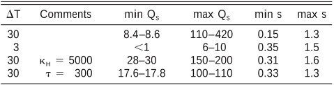 TABLE 4. Series of mixed BC experiments, asymmetric state. External parameters and some solution characteristics of the mixedboundary-condition runs. Min and max refer to minimum and maximum values for which an asymmetric state was found (not including slightly asymmetric states in DT 5 38 runs). Here, DT is in 8C, kH is in m2 s21, t is in days, and QS is in 1026 psu cm s21
 FIG. 5. Salt flux QS and imposed temperature difference DT for mixed-boundary-condition experiments with kH 5 1000 m2 s21. Locations in parameter space are denoted by a ‘‘1’’ if only T-dom states were found, by a ‘‘3’’ if only S-dom states were found, and by an ‘‘V’’ if at least one asymmetric state was found. Solid lines represent estimates of regime boundaries. Dotted lines are estimates of QS(DT ) for constant s values of 0.1, 0.1, 1, and 10 (section 4b). Here,Ï Ï s is the nondimensional subordinate hemisphere salinity gradient, normalized by its influence on density relative to DT.


