scispace - formally typeset
Search or ask a question
Journal ArticleDOI

Co-registration of surfaces by 3D least squares matching.

01 Mar 2010-Photogrammetric Engineering and Remote Sensing (American Society for Photogrammetry and Remote Sensing)-Vol. 76, Iss: 3, pp 307-318
TL;DR: In this paper, a method for automatic co-registration of 3D surfaces is presented, which utilizes the mathematical model of Least Squares 2D image matching and extends it for solving the 3D surface matching problem.
Abstract: A method for the automatic co-registration of 3D surfaces is presented. The method utilizes the mathematical model of Least Squares 2D image matching and extends it for solving the 3D surface matching problem. The transformation parameters of the search surfaces are estimated with respect to a template surface. The solution is achieved when the sum of the squares of the 3D spatial (Euclidean) distances between the surfaces are minimized. The parameter estimation is achieved using the Generalized Gauss-Markov model. Execution level implementation details are given. Apart from the co-registration of the point clouds generated from spaceborne, airborne and terrestrial sensors and techniques, the proposed method is also useful for change detection, 3D comparison, and quality assessment tasks. Experiments using terrain data examples show the capabilities of the method.

Summary (3 min read)

Introduction

  • With the availability of the various sensors and automated methods, the production of large numbers of point clouds is no longer particularly notable.
  • In terrestrial laser scanning practice, special targets provided by the vendors, e.g., Zoller Fröhlich, Leica, and Riegl, are mostly used for the co-registration of point clouds.
  • Such a strategy has several deficiencies with respect to fieldwork time, personnel and equipment costs, and accuracy.
  • In a recent study, Sternberg et al. (2004) reported that registration and geodetic measurements comprise 10 to 20 percent of the total project time.
  • In another study, a collapsed 1,000-car parking garage was documented in order to assess the damage and structural soundness of the building.

34980 Sile, Istanbul, Turkey, and formerly with the Institute of Geodesy and Photogrammetry, ETH Zurich,

  • Targets are essentially required in projects where the absolute orientation to an object coordinate system is needed.
  • The co-registration is crucially needed wherever spatially related data sets can be described as surfaces and has to be transformed to each other.
  • This work, called 3D Least Squares surface matching (LS3D), is another straightforward extension of the 2D Least Squares image matching and has the same underlying ideas and concepts.
  • The execution aspects and the implementation details are extensively elaborated.

Least Squares 3D Surface Matching

  • The Basic Estimation Model Two 3D surfaces are subject to a co-registration procedure.
  • This extension is especially useful to avoid such over-parameterization problems and for the flexible selection of the appropriate degree of freedom (DOF).
  • For every template surface element, the correspondence operator seeks a minimum Euclidean distance location on the search surface.
  • The central point is discarded according to the number of distances that are greater than a given distance threshold.
  • The mesh boundaries represent the model borders, and in addition the data holes inside the model.

Initialization: Defining the Box Size

  • For the sake of simplicity, they are given the same (M) here.
  • Step 2. Scan L1 and fill B. For any point ai, the box indices are as follows: (17) where stands for the truncation operator, and DX, DY, and DZ are dimensions of any box along the x y z axes, respectively.
  • In L2, the first point of the (u,v,w)th box is indexed by I while the address of the subsequent points is controlled using B whose value is incremented each time a new point enters the box.

Access Procedure

  • Step 1. Using Equation 17, compute the indices ui, vi, and wi of the box that contains point ai.
  • In L2, I indexes the first point, while the number of points in the box is given by the following formula: (19) The access procedure requires O(q) operations, where q is the average number of points in the box.
  • One of the main advantages of the boxing structure is a faster and easier access mechanism than the tree search-based methods provide.
  • In the LS3D surface matching case, the search surface, for which the boxing structure is established, is transformed to a new state by the current set of transformation parameters.
  • The access procedure is the same, except the following formula is used for the calculation of indices: (20) Where ‘ ’ stands for a vector dot product.

Simultaneous Matching of Surface Geometry and Intensity

  • When the object surface lacks sufficient geometric information, i.e., homogeneity or isotropicity of curvatures, the basic algorithm will either fail or will find a side minimum.
  • Available attribute information, e.g., intensity, color, temperature, etc., is used to form quasi-surfaces in addition to the actual ones.
  • The matching is performed by simultaneous use of surface geometry and attribute information under a combined estimation model (Akca, 2007a).

Experimental Results

  • The algorithm was implemented as a stand-alone MS Windows™ application with a graphical user interface.
  • The software package was developed with the C/C programming language.
  • Thus, angle was excluded from the system, and the second version of the computation was run in 5-DOF mode.
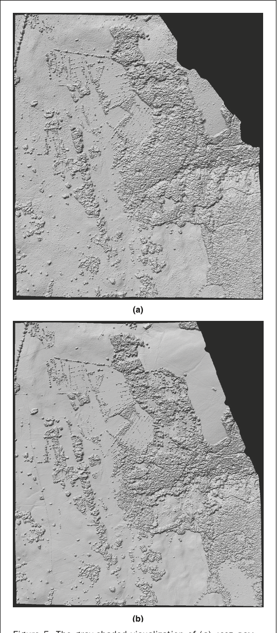
  • (a) SRTM C-Band DEM with data holes, (b) registration of a local DEM onto the SRTM C-Band DEM by use of the LS3D matching, and (c) filled data holes.

Image Data

  • The image data consisted of 28 DMC images with a ground sampling distance (GSD) of 22 cm arranged in four parallel flight strips in the E/W direction, each of seven images.
  • The forward and side overlap of the DMC images were 60 percent and 75 percent, respectively.
  • The automated DSM generation was performed using the SAT-PP software 314 March 2010 PHOTOGRAMMETRIC ENGINEER ING & REMOTE SENS ING TABLE 3.

DSM Comparison and Analysis

  • Evaluation is done based on the height differences.
  • The LS3D surface matching method was used to avoid both these shortcomings.
  • This is actually the difference between the two DSMs after removing the reference frame differences.
  • In planimetry, this bias is due to the different orientations of the images and the lidar, and is significant only in the Y (N/S) direction.
  • The study is a cooperative project between the IGP and the Department of Landscape Inventories of the Swiss Federal Research Institute WSL.

75 percent forward and a 30 percent lateral overlap.

  • All images were digitized with a Vexcel UltraScan® scanner with a 15 micron pixel size, which results in a GSD of 15 cm and 8.25 cm for the 1997 and 2002 images, respectively.
  • The 1997 film images had severe scratches on the emulsion side, causing artifacts in the digitized images and DSM errors in the automated DSM generation .
  • The national lidar data of the Swiss Federal Office of Topography was acquired in 2001 when leaves were off the trees.
  • The first pulse point cloud was interpolated to a regular grid with 2.5 m grid spacing, called 2001_DSM.

Co-registration and Change Detection

  • They cannot consider the surface modeling errors.
  • The estimation model is the Generalized Gauss-Markov model.
  • The capability to match surfaces of different quality and resolution is another positive aspect of the proposed method.
  • This is especially useful for quality assessment and change detection tasks as discussed in the Experimental Results Section.

Acknowledgments

  • I would like to express my gratitude to my advisor, Professor Armin Gruen, for his invaluable advice and support on the work presented here.
  • The author is financially supported by an ETHZ internal research grant, which is gratefully acknowledged.

Conclusions

  • The basic estimation model is a generalization of the Least Squares matching concept.
  • The current implementation uses a 3D similarity transformation model for the geometric relationship.
  • The unknown transformation parameters are treated as observables with proper weights, so that sub-versions of the 7-parameter model can be run, i.e., rigid body (6-DOF), tilt and translation (5-DOF), translation (3-DOF), horizontal shift (2-DOF), and depth (1-DOF).

Did you find this useful? Give us your feedback

Content maybe subject to copyright    Report

Abstract
A method for the automatic co-registration of 3D surfaces is
presented. The method utilizes the mathematical model of
Least Squares
2D image matching and extends it for solving
the
3D surface matching problem. The transformation param-
eters of the search surfaces are estimated with respect to a
template surface. The solution is achieved when the sum of
the squares of the
3D spatial (Euclidean) distances between
the surfaces are minimized. The parameter estimation is
achieved using the Generalized Gauss-Markov model. Execu-
tion level implementation details are given. Apart from the
co-registration of the point clouds generated from spaceborne,
airborne and terrestrial sensors and techniques, the proposed
method is also useful for change detection,
3D comparison,
and quality assessment tasks. Experiments using terrain data
examples show the capabilities of the method.
Introduction
With the availability of the various sensors and automated
methods, the production of large numbers of point clouds is
no longer particularly notable. In many cases, the object of
interest is covered by a number of point clouds, which are
referenced in different spatial or temporal datums. Therefore,
the issue of co-registration of point clouds (or surfaces) is an
essential topic in
3D modeling.
In terrestrial laser scanning practice, special targets
provided by the vendors, e.g., ZollerFröhlich, Leica, and
Riegl, are mostly used for the co-registration of point clouds.
However, such a strategy has several deficiencies with
respect to fieldwork time, personnel and equipment costs,
and accuracy. In a recent study, Sternberg et al. (2004)
reported that registration and geodetic measurements com-
prise 10 to 20 percent of the total project time. In another
study, a collapsed 1,000-car parking garage was documented
in order to assess the damage and structural soundness of the
building. The laser scanning took three days, while the
conventional survey of the control points required two days
(Greaves, 2005). In a project conducted by our research group
at Pinchango Alto (Lambers et al., 2007), two persons set the
targets in the field and measured them using the real-time
kinematic
GPS technique in one and one-half days.
As well as fieldwork time, accuracy is another impor-
tant concern. The target-based registration methods may not
exploit the full accuracy potential of the data. The geodetic
measurements naturally introduce some error, which might
exceed the internal error of the scanner instrument. In
PHOTOGRAMMETRIC ENGINEERING & REMOTE SENSING
March 2010 307
Department of Information Technologies, Isik University,
34980 Sile, Istanbul, Turkey, and formerly with the Institute
of Geodesy and Photogrammetry, ETH Zurich,
Switzerland (akca@isikun.edu.tr).
Photogrammetric Engineering & Remote Sensing
Vol. 76, No. 3, March 2010, pp. 307–318.
0099-1112/10/7603–0307/$3.00/0
© 2010 American Society for Photogrammetry
and Remote Sensing
Co-registration of Surfaces by
3D Least Squares Matching
Devrim Akca
addition, the targets must be kept stable during the whole of
the data acquisition campaign. This might be inconvenient
when the scanning work stretches over more than one day.
On the other hand, one important advantage of the target
based methods should not be ignored. Targets are essentially
required in projects where the absolute orientation to an
object coordinate system is needed.
The surface based registration techniques stand as
efficient and versatile alternatives to the target-based tech-
niques. They simply bring the strenuous additional fieldwork
of the registration task to the computer in the office, at the
same time optimizing the project cost and duration, and
achieving a better accuracy. In the last decade, surface-based
registration techniques have been studied extensively. The
large number of research activities on the topic demonstrates
the relevance of the problem. For an exhaustive literature
review, we refer to Gruen and Akca (2005).
The co-registration is crucially needed wherever spatially
related data sets can be described as surfaces and has to be
transformed to each other. Examples can be found in medicine,
computer graphics, animation, cartography, virtual reality,
industrial inspection and quality control, change detection,
spatial data fusion, cultural heritage, photogrammetry, etc.
We treat the co-registration problem as a Least Squares
matching of overlapping surfaces. Least Squares matching is
a mathematical concept, which was originally developed
for automatic point transfer on stereo or multiple images
(Ackermann, 1984; Pertl, 1984; Gruen, 1985). More recently,
it has been extended to many problem-specific cases, e.g.,
3D voxel matching (Maas and Gruen, 1995) and the line
feature extraction techniques (Gruen, 1996).
This work, called
3D Least Squares surface matching
(
LS3D), is another straightforward extension of the 2D Least
Squares image matching and has the same underlying ideas
and concepts. The next section introduces the basic estima-
tion model. The execution aspects and the implementation
details are extensively elaborated. Particular attention is
given to the surface-to-surface correspondence search, outlier
detection, and the computational acceleration. In previous
work, examples covering the co-registration of the terrestrial
laser scanning data sets were given (Gruen and Akca, 2005;
Akca, 2007a). In the work presented here, the experimenta-
tion concentrates on the topographic data sets, mostly
generated by use of photogrammetric and airborne lidar
techniques. Apart from the co-registration of point clouds, the
proposed method can be utilized for many types of geo-data

308 March 2010
PHOTOGRAMMETRIC ENGINEERING & REMOTE SENSING
analyses. The experiments given in the third section show
examples of how the
3D surface matcher performs more
advantageously than the conventional methods for change
detection and quality assessment tasks.
Least Squares 3D Surface Matching
The Basic Estimation Model
Two 3D surfaces are subject to a co-registration procedure.
The search surface g (x, y, z) is going to be transformed to
the spatial domain of the template surface f (x, y, z). Both f
(x, y, z) and g (x, y, z) are piecewise discrete representa-
tions of the continuous function of the object surface. In
the current implementation, a triangular mesh or a grid
mesh type of representation is used. In the case of the
triangular mesh representation, the piecewise surface is
composed of planar triangle elements; in the same manner,
the grid mesh representation is composed of bi-linear grid
surface elements.
Surface topology is established simply by loading the
data files, e.g., range scanner point clouds or photogrammetric
digital elevation models (
DEM), in row or column order. The
point spacing is by definition irregular, wherefore the regular
grid
DEM is an under-capability case.
Every template surface element is matched to a conjugate
search surface element to establish the surface-to-surface
correspondence. This is achieved by a correspondence
operator. Occlusions and outliers are the perturbation cases,
which are excluded from the system automatically. While all
template surface elements are sought by the operator, some
of the search surface elements might not coincide at all.
If a matching is established between the two surface
elements f (x, y, z) and g (x, y, z), the following equation
holds:
(1)
where e (x, y, z) is a true error vector covering the random
errors of the template and search surfaces, which are
assumed to be uncorrelated. Equation 1 is the observation
equation, which is set up for each template element that
has a valid surface match. The transformation parameters
of the search surface g (x, y, z) are variables to be
estimated.
Here, we have a peculiar case where the search surface
g (x, y, z) is not analytically continuous; rather it is composed
of discrete finite elements in the form of planar triangles or
bilinear grids. As a consequence, the mathematical derivation
operation cannot be performed analytically.
Equation 1 is non-linear. It is linearized by the Taylor
Series expansion:
(2)
with notations:
(3)
where the terms g
x
, g
y
, and g
z
are the numerical first
derivatives of the function g (x, y, z), which are defined
as the components of the local surface normal vector n.
Their calculation depends on the analytical representation
of the search surface elements, i.e., planar triangles or
bilinear grids. The derivative terms are given as the x-y-z
g
x
0g
0
(x, y, z)
0x
,
g
y
0g
0
(x, y, z)
0y
,
g
z
0g
0
(x, y, z)
0z
0g
0
(x, y, z)
0z
dz (f(x, y, z) g
0
(x, y, z))
e(x, y, z)
0g
0
(x, y, z)
0x
dx
0g
0
(x, y, z)
0y
dy
f(x, y, z) e(x, y, z) g(x, y, z)
components of the local normal vectors, which are com-
puted at the exact matching location on the respective
search surface elements:
[g
x
g
y
g
z
]
T
n [n
x
n
y
n
z
]
T
. (4)
The terms dx, dy, and dz are the differentiation terms of the
selected
3D transformation model. The geometric relation-
ship is established with a seven-parameter
3D similarity
transformation whose differentiation gives:
(5)
where a
ij
are the coefficient terms. Their expansions are
given in Akca (2007b). The vector [t
x
t
y
t
z
]
T
is the translation
vector, the scalar m is the uniform scale factor, and the
angles
,
, and
are the elements of the orthogonal rotation
matrix R. Depending on the characteristics of the template
and search surfaces, any other higher order transformation
model, e.g., a
3D affine or polynomial model, can be chosen.
By substituting Equations 3 and 5, Equation 2 gives the
following form:
(6)
where g
0
(x, y, z) is the coarsely aligned search surface. The
coarse alignment is performed using the initial approxima-
tions of the transformation parameters (t
0
x
, t
0
y
, t
0
z
, m
0
,
0
,
0
,
and
0
). The term f (x, y, z) g
0
(x, y, z) denotes the Euclid-
ean distance between the template and the corresponding
search surface elements.
Equation 6 gives in matrix notation:
(7)
Where A is the design matrix, x [dt
x
dt
y
dt
z
dm d
d
d
]
T
is the parameter vector, P P
ll
is the priori weight
coefficient matrix, and l f (x, y, z) g
0
(x, y, z) is the
discrepancy vector.
With the statistical expectation operator E and the
assumptions
, (8)
the system (Equation 7) is a Gauss-Markov estimation model.
The unknown parameters are introduced into the system as
fictitious observations:
(9)
where I is the identity matrix, l
b
is the (fictitious) observa-
tion vector, and P
b
is the associated weight coefficient
matrix. By selecting a very large weight value ((P
b
)
ii
: ), an
individual parameter can be assigned as constant. In com-
monly used topographic data sets, scale differences, even in
some cases the rotational differences do not occur. This
extension is especially useful to avoid such over-parameteri-
zation problems and for the flexible selection of the appro-
priate degree of freedom (
DOF).
The joint system of Equations 7 and 9 is a Generalized
Gauss-Markov model. The Least Squares solution gives the
e
b
Ix l
b
, P
b
E(e) 0, E1ee
T
2 s
0
2
P
1
e Ax l, P
(f (x, y,z) g
0
(x,y, z))
(g
x
a
13
g
y
a
23
g
z
a
33
)dk
(g
x
a
12
g
y
a
22
g
z
a
32
)dw
(g
x
a
11
g
y
a
21
g
z
a
31
)dv
(g
x
a
10
g
y
a
20
g
z
a
30
)dm
e(x,y,z) g
x
dt
x
g
y
dt
y
g
z
dt
z
J
d x
d y
dz
K
J
d t
x
d t
y
dt
z
K
d m
J
a
10
a
20
a
30
K
J
a
11
a
12
a
13
a
21
a
22
a
23
a
31
a
32
a
33
KJ
d v
d w
d k
K

PHOTOGRAMMETRIC ENGINEERING & REMOTE SENSING
March 2010 309
estimated parameter vector and the variance factor as in the
following equations:
(10)
(11)
where stands for the Least Squares estimator, r is the
system redundancy, and the residual vectors v and v
b
are
the Least Squares estimation of the true error vectors e and
e
b
, respectively.
The solution is iterative. At the end of each iteration,
the search surface is transformed to a new state using the
updated set of transformation parameters:
(12)
(13)
. (14)
At each iteration, the design matrix A and the discrep-
ancies vector l are re-evaluated. The iteration stops if each
element of the vector falls below a certain limit:
(15)
where the criteria c
i
is selected as 1 ppm (10
6
) for the
scale factor, between 1/10 and 1/100 of the least significant
digit for the translation elements, and 10
3
grad for the
rotation elements.
The functional model is non-linear; thus, the initial
approximations of the parameters are required. The initial
approximations should be given or should be computed
prior to the matching. In this paper, the experiments use
geo-datasets, which are crudely aligned. Thus, the initial
approximations of the rotation and translation parameters
are assumed to be zero. This might not be the case for the
terrestrial laser scanning point clouds. In such cases, the
initial approximations can be provided by interactively
selecting three common points on both surfaces before
the matching.
Correspondence Search
For every template surface element, the correspondence
operator seeks a minimum Euclidean distance location on
the search surface. The template surface elements are
represented by the data points. Accordingly, the procedure
becomes a point-to-plane distance or point-to-bilinear
surface distance computation. When a minimum Euclidean
distance is found, in a subsequent step the matching point is
tested to determine whether it is located inside the search
surface element (point-in-polygon test). If not, this element
is disregarded and the operator moves to the next search
surface element with the minimum distance. Hypothetically,
the correspondence criterion searches a minimum magnitude
vector that is perpendicular to the search surface element
and passes through the template point.
In the most straightforward case, the computational
complexity is of order O(N
t
N
s
), where N
t
is the number of
template elements and N
s
is the number of search elements.
This computational expense is reduced by constricting the
search space within
3D boxes. The details are given in the
Computational Acceleration sub-section.
Outlier Detection and Reliability Aspects
Detection of the false correspondences with respect to the
outliers and occlusions is a crucial part of every surface
ƒ
dp
i
ƒ
6 c
i
, dp
i
{dt
x
, dt
y
, dt
z
, dm, dv, dw, dk}
x
N
[vwk]
T
[v
0
w
0
k
0
]
T
[d
N
v d
N
w
d
N
k
]
T
m m
0
d
N
m
[t
x
t
y
t
z
]
T
[t
0
x
t
0
y
t
0
z
]
T
[d
N
t
x
d
N
t
y
d
N
t
z
]
T
N
s
N
0
2
v
T
Pv v
b
T
P
b
v
b
r
N
x (A
T
PA P
b
)
1
(A
T
Pl P
b
l
b
)
matching method. We use the following strategies in order
to localize and eliminate the outliers and the occluded parts.
A median type of filtering is applied prior to the
matching. For each point, the distances between the
central point and its k-neighborhood points are calculated.
In our implementation, k is selected as 8. If most of those
k-distance values are much greater than the average point
density, the central point is likely to be an erroneous
point on a poorly reflecting surface (e.g., window or glass)
or a range artifact due to surface discontinuity (e.g., points
on the object silhouette). The central point is discarded
according to the number of distances that are greater than
a given distance threshold.
In the course of iterations, a simple weighting scheme
adapted from the robust estimation methods is used:
(16)
The constant value K can be altered according to the
task. If it is an ordinary surface co-registration task, it
should be set to a high value (e.g., K 8 or 10) to reduce
type I errors confidently. Because of the high redundancy of
a typical data set, a certain number of occlusions and/or
smaller outliers, i.e., type II errors, do not have significant
effects on the estimated parameters. If it is a change detec-
tion or deformation study, the constant value K should be
selected based on the a priori knowledge in order that the
changed or deformed parts are excluded from the estimation.
Finally, the correspondences coinciding with mesh
boundaries are excluded from the estimation. The mesh
boundaries represent the model borders, and in addition the
data holes inside the model. The data holes are possibly due
to occlusions. Rejecting the surface correspondences on the
mesh boundaries effectively eliminates the occlusions.
Precision
The quality of the estimated parameters can be checked
through the a posteriori co-variance matrix.
The theoretical precisions of the transformation parame-
ters are optimistic, mainly due to the stochastic properties
of the search surfaces that have not been considered as
such in the estimation model, as is typically done in Least
Squares matching (Gruen, 1985). The omissions are expected
to be minor and do not disturb the solution vector signifi-
cantly. However, the a posteriori covariance matrix will be
affected by the neglected uncertainty of the function values
g (x, y, z). This causes deterioration in the realistic precision
estimates. More details on this issue can be found in Gruen
(1985), Maas (2002), Gruen and Akca (2005), and Kraus
et al. (2006).
Computational Acceleration
Searching for correspondence is guided by an efficient boxing
algorithm (Chetverikov, 1991), which partitions the search
space into voxels. For a given surface element, the correspon-
dence is searched only in the box containing this element
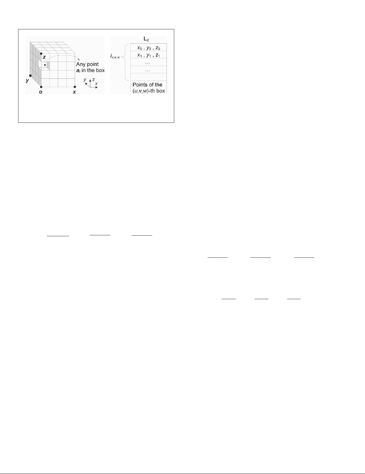
and in the adjacent boxes (Figure 1a). The original publica-
tion concerned
2D point sets. It is straightforwardly extended
here to the
3D case.
Let points a
i
= {x
i
, y
i
, z
i
} S, i 0, 1,..., N
s
1,
represent the object S
3
, and be kept in list L
1
in
spatially non-ordered form. The boxing data structure
consists of a rearranged point list L
2
and an index matrix
I I
u, v, w
whose elements are associated with individual
boxes: u,v,w 0,1, ..., M 1. The items of L
2
are the
coordinates of N
s
points placed in the order of boxes. The
index matrix I contains integers indicating the beginnings of
the boxes in L
2
(Figure 1b).
1P2
ii
e
1if|1v2
i
|6 K
N
s
0
0 else

310 March 2010
PHOTOGRAMMETRIC ENGINEERING & REMOTE SENSING
(a) (b)
Figure 1. (a) The 3D boxing bounds all the data points,
and (b) The boxing data structure.
Initialization: Defining the Box Size
Step 1. Recall min, max{x
i
, y
i
, z
i
} of data volume.
Step 2. Define the number of boxes along the xyz
axes. For the sake of simplicity, they are given
the same (M) here.
Pass 1: Computing I
Step 1. Allocate an M M M size accumulator array
B B
u,v,w
, which is to contain the number of
points in each box.
Step 2. Scan L
1
and fill B. For any point a
i
, the box
indices are as follows:
(17)
where stands for the truncation operator, and D
X
, D
Y
,
and D
Z
are dimensions of any box along the xyz axes,
respectively.
Step 3. Fill I using the following recursive formula: I
0,0,0
= 0.
For all
(18)
Pass 2: Filling L
2
Step 1. For all u, v, and w, set B
u,v,w
0.
Step 2. Scan L
1
again. Use Equation 17, I and B to fill
L
2
. In L
2
, the first point of the (u,v,w)
th
box is
indexed by I while the address of the subse-
quent points is controlled using B whose value
is incremented each time a new point enters the
box. Finally, release the memory area of B.
The memory requirement is of order O(N
s
) for L
2
and
O(M
3
) for I. For the sake of clarity of the explanation, L
2
is
given as a point list containing the x-y-z coordinate values. If
one wants to keep the L
1
in the memory, then L
2
should only
contain the access indices to L
1
or pointers, which directly
point to the memory locations of the point coordinates.
Access Procedure
Step 1. Using Equation 17, compute the indices u
i
, v
i
,
and w
i
of the box that contains point a
i
.
I
u, v, w
L
I
u, v, w1
B
u, v, w1
if w 7 0
I
u, v1, M1
B
u, v1, M1
else if v 7 0
I
u1, M1, M1
B
u1, M1, M1
else
(u,v,w) Z (0,0,0)
;:
u
i
j
x
i
x
min
D
X
k
, v
i
j
y
i
y
min
D
Y
k
, w
i
j
z
i
z
min
D
Z
k
Step 2. Use the boxing structure to retrieve the points
bounded by the (u,v,w)
th
box. In L
2
, I indexes
the first point, while the number of points in
the box is given by the following formula:
(19)
The access procedure requires O(q) operations, where
q is the average number of points in the box. One of the
main advantages of the boxing structure is a faster and
easier access mechanism than the tree search-based
methods provide. Construction time of the boxing method
O(N
s
) is less than what the tree search methods need, i.e.,
order of O(N
s
logN
s
) for a k-D tree (Greenspan and Yurick,
2003; Arya and Mount, 2005). On the other hand, the tree
search methods obviously need less storage space, which
is only order of O(N
s
).
The boxing structure, and in general all search struc-
tures, are designed for searching the nearest neighborhood in
the static point clouds. In the
LS3D surface matching case,
the search surface, for which the boxing structure is estab-
lished, is transformed to a new state by the current set of
transformation parameters. Nevertheless, there is no need
either to re-establish the boxing structure or to update the
I and L
2
in each iteration. Only the positions of those four
points (Figure 1a) are updated in the course of iterations:
o {x
min
, y
min
, z
min
}, x {x
max
, y
min
, z
min
}, y {x
min
, y
max
,
z
min
}, z {x
min
, y
min
, z
max
}. They uniquely define the boxing
structure under the similarity transformation. The access
procedure is the same, except the following formula is used
for the calculation of indices:
(20)
Where ‘’ stands for a vector dot product. If the transforma-
tion is a similarity rather than a rigid body, the D
X
, D
Y
, and
D
Z
values must also be updated in the iterations:
. (21)
In the current implementation, the correspondence
is searched in the boxing structure during the first few
iterations, and at the same time, its evolution is tracked
across the iterations. Afterwards, the searching process is
carried out only in an adaptive local neighborhood accord-
ing to the previous position and change of correspondence.
In any step of the iteration, if the change of correspondence
for a surface element exceeds a limit value, or oscillates,
the search procedure for this element is returned to the
boxing structure again.
Algorithmic Extensions
Multiple Surface Matching
When more than two point clouds with multiple overlaps
exist, a two step solution is adopted. First, the pairwise
LS3D matchings are run on every overlapping pair and a
subset of point correspondences is saved to separate files.
In the global registration step, all these files are passed to a
block adjustment by the independent models procedure
(Ackermann et al., 1973), which is a well known orienta-
tion procedure in photogrammetry. More details can be
found in Akca (2007b).
D
X
ox
M
, D
Y
oy
M
, D
Z
oz
M
u
i
j
oa
i
#
ox
ox
D
X
k
, v
i
j
oa
i
#
oy
oy
D
Y
k
, w
i
j
oa
i
#
oz
oz
D
Z
k
L
I
u, v, w1
I
u, v, w
if w 6 M 1
I
u, v1, 0
I
u, v, M1
else if v 6 M 1
I
u1, 0, 0
I
u, M1, M1
else if u 6 M 1
N
s
I
M1, M1, M1
else

PHOTOGRAMMETRIC ENGINEERING & REMOTE SENSING
March 2010 311
(a)
(b)
(c)
(d)
Figure 2. Experiment “Tucume”: (a) The shaded view of the final composite surface after
the
LS
3
D
surface matching. Note that the overlapping area is delineated by gray borderlines.
The residuals between the fixed and transformed surfaces are shown; (b) after the
LS
3
D
matching; and (c) after the
ICP
matching. The residuals bar unit (d) is in meters.
Simultaneous Matching of Surface Geometry and Intensity
When the object surface lacks sufficient geometric informa-
tion, i.e., homogeneity or isotropicity of curvatures, the basic
algorithm will either fail or will find a side minimum. In this
extension, available attribute information, e.g., intensity,
color, temperature, etc., is used to form quasi-surfaces in
addition to the actual ones. The matching is performed by
simultaneous use of surface geometry and attribute informa-
tion under a combined estimation model (Akca, 2007a).
Further Conceptual Extensions
The further conceptual extensions are given as: the Least
Squares matching of
3D curves, matching of 3D curves or 3D
sparse points (e.g., ground control points) with a 3D surface,
and a general framework, which can perform the multiple
surface matching, the combined surface geometry and
intensity matching, and georeferencing tasks simultaneously
(Akca, 2007b).
Experimental Results
The algorithm was implemented as a stand-alone MS
Windows
application with a graphical user interface.
The software package was developed with the C/C⫹⫹
programming language. The presented examples use solely
the basic model, not the algorithmic extensions.
Tucume
The first experiment is the matching of two photogrammetri-
cally derived digital terrain models (
DTM) of an area in
Tucume (Peru). The horizontal resolution of the
DTMs was
5 m. The
DTMs were manually measured as two independent
models from 1:10 000 scale B/W aerial images in one strip
with an overlap of 60 percent in the flight direction. More
details are given in Sauerbier et al. (2004).
Although it is only a
2.5D model, it is a good example of
the weak data configuration case since the overlapping area is
relatively narrow (along the Y-axis) with little information
regarding the surface geometry (Figure 2a). The
LS3D algorithm
was run in
6-DOF mode with three translation and three
rotation parameters. This version showed a large correlation
coefficient 0.99 between the t
y
and angle, which is an over-
parameterization case. Thus, angle was excluded from the
system, and the second version of the computation was run in
5-DOF mode. The results are successful (Table 1). The compu-
tation takes 1.9 and 2.5 seconds for the plane surface (P) and
bi-linear surface (B) representation versions, respectively.
The ratio between the standard deviations of
and
angles is by factor 14. This difference in angular uncertainty
is due to difference in overlapping areas along the X and Y
axes. The residuals between the fixed and transformed
surfaces show a random distribution pattern, except for some
occasional measurement and modeling errors (Figure 2b).

Citations
More filters
Journal ArticleDOI
TL;DR: In this article, a procedure to fuse automatically generated infrared mosaics and visible images to combine geometric information with thermal data in the same image is described, where the fused images are then used for the automatic generation of a thermographic 3D model of the building through image matching, where apart from having thermographic information available, geometric measurements can be performed.

71 citations

Journal ArticleDOI
TL;DR: In this article, a remote sensing-based approach for detailed topographic investigations in steep periglacial high-mountain faces was described, where a time series of high-resolution digital terrain models (DTMs) with a 2m resolution was produced from digital aerial photogrammetry for 1956, 1988 and 2001 and from airborne LiDAR for 2005 and 2007.
Abstract: This paper describes a remote sensing-based approach for detailed topographic investigations in steep periglacial high-mountain faces. The study was conducted at one of the highest periglacial rock faces in the European Alps, the permafrost-affected and partially glacierised east face of Monte Rosa. Strongly increased rock and ice avalanche activity on this rock wall has caused major topographic change in recent decades. A time series of high-resolution digital terrain models (DTMs) with a 2-m resolution was produced from digital aerial photogrammetry for 1956, 1988 and 2001 and from airborne LiDAR for 2005 and 2007. The DTM comparisons reveal a total volume loss of permafrost-affected bedrock and glacier ice of more than 20 × 106 m3 over the past 50 years, with the majority of the loss since 1988. Analysis of all unstable areas and detachment zones showed that the sequence of the main slope failures is spatially connected and that there is coupling between permafrost bedrock instability and the condition of adjacent hanging glaciers. Copyright © 2011 John Wiley & Sons, Ltd.

68 citations


Cites methods from "Co-registration of surfaces by 3D l..."

  • ...Consequently, the LiDAR DTM acquired in 2007 was taken as the reference surface for all the other processed DTMs. Automatic co-registration of the DTMs on the reference DTM was conducted with LS3D (Least Squares 3D Matching software; Akca, 2010)....

    [...]

  • ...The DTM difference calculations in LS3D yielded a direct estimate of the location and amount of topographic change over the four time periods (Figure 6)....

    [...]

  • ...Automatic co-registration of the DTMs on the reference DTM was conducted with LS3D (Least Squares 3D Matching software; Akca, 2010)....

    [...]

  • ...The transformation of individual DTMs to a common reference system using LS3D reduced the offsets between DTMs that were introduced by slightly different GPS positions....

    [...]

Journal ArticleDOI
TL;DR: The proposed method for the quality control of three‐dimensional building models can favourably address the reference system accuracy, positional accuracy and completeness.
Abstract: This project has been funded by Ordnance Survey Research, the research and development department of the Ordnance Survey of Great Britain, which is gratefully acknowledged. The first author, Devrim Akca, was formerly with the Institute of Geodesy and Photogrammetry of ETH Zurich, Switzerland

60 citations


Cites background or methods from "Co-registration of surfaces by 3D l..."

  • ...The input model is co-registered to the verification data by use of the least squares 3D surface matching (LS3D) method (Gruen and Akca, 2005; Akca, 2010)....

    [...]

  • ...See Akca and Gruen (2005) and Akca (2007; 2010) for the details....

    [...]

  • ...Recently, it has also been used for 3D comparison, change detection, quality inspection and validation studies (Akca, 2007; 2010)....

    [...]

Journal ArticleDOI
TL;DR: An automated processing method for plot-level stem mapping that matches multiple scans without artificial references that makes stem mapping more reliable and consistent among plots, reduces the costs associated with plot-based stem mapping, and enhances the efficiency.

53 citations


Cites methods from "Co-registration of surfaces by 3D l..."

  • ...A number of automated registration methods have been develped to register multiple scans (Besl and McKay, 1992; Rabbani t al., 2007; Henning and Radtke, 2008; Akca, 2010; Canaz and abib, 2013; Kelbe, 2015)....

    [...]

Journal ArticleDOI
TL;DR: In this article, the authors compare the significance of spatially variable versus spatially uniform digital elevation models (DEMs) errors on change detection by thresholding the DEM of Difference at a 95% confidence interval (2σ).

53 citations

References
More filters
Journal ArticleDOI
Paul J. Besl1, H.D. McKay1
TL;DR: In this paper, the authors describe a general-purpose representation-independent method for the accurate and computationally efficient registration of 3D shapes including free-form curves and surfaces, based on the iterative closest point (ICP) algorithm, which requires only a procedure to find the closest point on a geometric entity to a given point.
Abstract: The authors describe a general-purpose, representation-independent method for the accurate and computationally efficient registration of 3-D shapes including free-form curves and surfaces. The method handles the full six degrees of freedom and is based on the iterative closest point (ICP) algorithm, which requires only a procedure to find the closest point on a geometric entity to a given point. The ICP algorithm always converges monotonically to the nearest local minimum of a mean-square distance metric, and the rate of convergence is rapid during the first few iterations. Therefore, given an adequate set of initial rotations and translations for a particular class of objects with a certain level of 'shape complexity', one can globally minimize the mean-square distance metric over all six degrees of freedom by testing each initial registration. One important application of this method is to register sensed data from unfixtured rigid objects with an ideal geometric model, prior to shape inspection. Experimental results show the capabilities of the registration algorithm on point sets, curves, and surfaces. >

17,598 citations

Journal ArticleDOI
TL;DR: A new approach is proposed which works on range data directly and registers successive views with enough overlapping area to get an accurate transformation between views and is performed by minimizing a functional which does not require point-to-point matches.

2,850 citations


"Co-registration of surfaces by 3D l..." refers methods in this paper

  • ...A comparison study between the LS3D and the Iterative Closest Point (ICP; introduced by Besl and McKay (1992), Chen and Medioni (1992), and Zhang (1994) was carried out....

    [...]

Journal ArticleDOI
TL;DR: A heuristic method has been developed for registering two sets of 3-D curves obtained by using an edge-based stereo system, or two dense3-D maps obtained by use a correlation-based stereoscopic system, and it is efficient and robust, and yields an accurate motion estimate.
Abstract: A heuristic method has been developed for registering two sets of 3-D curves obtained by using an edge-based stereo system, or two dense 3-D maps obtained by using a correlation-based stereo system. Geometric matching in general is a difficult unsolved problem in computer vision. Fortunately, in many practical applications, some a priori knowledge exists which considerably simplifies the problem. In visual navigation, for example, the motion between successive positions is usually approximately known. From this initial estimate, our algorithm computes observer motion with very good precision, which is required for environment modeling (e.g., building a Digital Elevation Map). Objects are represented by a set of 3-D points, which are considered as the samples of a surface. No constraint is imposed on the form of the objects. The proposed algorithm is based on iteratively matching points in one set to the closest points in the other. A statistical method based on the distance distribution is used to deal with outliers, occlusion, appearance and disappearance, which allows us to do subset-subset matching. A least-squares technique is used to estimate 3-D motion from the point correspondences, which reduces the average distance between points in the two sets. Both synthetic and real data have been used to test the algorithm, and the results show that it is efficient and robust, and yields an accurate motion estimate.

2,177 citations


"Co-registration of surfaces by 3D l..." refers methods in this paper

  • ...A comparison study between the LS3D and the Iterative Closest Point (ICP; introduced by Besl and McKay (1992), Chen and Medioni (1992), and Zhang (1994) was carried out....

    [...]

01 Jan 1992
TL;DR: In this article, a least-squares technique is used to estimate 3D motion from the point correspondences, which reduces the average distance between curves in two sets, and yields an accurate motion estimate.
Abstract: Geometric matching in general is a difficult unsolved problem in computer vision. Fortunately, in many pratical applications, some a priori knowledge exists which considerably simplifies the problem. In visual navigation, for example, the motion between successive positions is usually either small or approximately known, but a more precise registration is required for environment modeling. The algorithm described in this report meets this need. Objects are represented by free-form curves, i.e., arbitrary spaces curves of the type found in practice. A curve is available in the form of a set of chained points. The proposed algorithm is based on iteratively matching points on one curve to the closest points on the other. A least-squares technique is used to estimate 3-D motion from the point correspondences, which reduces the average distance between curves in two sets. Both synthetic and real data have been used to test the algorithm, and the results show that it is efficient and robust, and yields an accurate motion estimate. The algorithm can be easily extended to solve similar problems such as 2-D curve matching and 3-D surface matching.

1,986 citations

01 Jan 1985
TL;DR: In this article, the adaptive least square correlation (ALES) is used for image matching, which allows for simultaneous radiometric corrections and local geometrical image shaping, whereby the system parameters are automatically assessed, corrected, and thus optimized during the least squares iterations.
Abstract: The Adaptive Least Squares Correlation is a very potent and flexible technique for all kinds of data matching problems. Here its application to image matching is outlined. It allows for simultaneous radiometric corrections and local geometrical image shaping, whereby the system parameters are automatically assessed, corrected, and thus optimized during the least squares iterations. The various tools of least squares estimation can be favourably utilized for the assessment of the correlation quality. Furthermore, the system allows for stabilization and improvement of the correlation procedure through the simultaneous consideration of geometrical constraints, e.g. the collinearity condition. Some exciting new perspectives are emphasized, as for example multiphoto correlation, multitemporal and multisensor correlation, multipoint correlation, and simultaneous correlation/triangulation.

667 citations


"Co-registration of surfaces by 3D l..." refers background in this paper

  • ...More details on this issue can be found in Gruen (1985), Maas (2002), Gruen and Akca (2005), and Kraus et al. (2006)....

    [...]

  • ...Least Squares matching is a mathematical concept, which was originally developed for automatic point transfer on stereo or multiple images (Ackermann, 1984; Pertl, 1984; Gruen, 1985)....

    [...]

  • ...The theoretical precisions of the transformation parameters are optimistic, mainly due to the stochastic properties of the search surfaces that have not been considered as such in the estimation model, as is typically done in Least Squares matching (Gruen, 1985)....

    [...]

Frequently Asked Questions (2)
Q1. What are the contributions mentioned in the paper "Co-registration of surfaces by 3d least squares matching" ?

A method for the automatic co-registration of 3D surfaces is presented. In a recent study, Sternberg et al. ( 2004 ) reported that registration and geodetic measurements comprise 10 to 20 percent of the total project time. The geodetic measurements naturally introduce some error, which might exceed the internal error of the scanner instrument. The target-based registration methods may not exploit the full accuracy potential of the data. 

The further conceptual extensions are given as: the Least Squares matching of 3D curves, matching of 3D curves or 3D sparse points ( e. g., ground control points ) with a 3D surface, and a general framework, which can perform the multiple surface matching, the combined surface geometry and intensity matching, and georeferencing tasks simultaneously ( Akca, 2007b ).