scispace - formally typeset
Open AccessProceedings ArticleDOI

Cross-modal localization through mutual information

Reads0
Chats0
TLDR
This paper presents an approach to localise this embedded common information through an indirect method of estimating mutual information between all signal sources, which leads to faster convergence with much reduced spurious associations.
Abstract
Relating information originating from disparate sensors observing a given scene is a challenging task, particularly when an appropriate model of the environment or the behaviour of any particular object within it is not available. One possible strategy to address this task is to examine whether the sensor outputs contain information which can be attributed to a common cause. In this paper, we present an approach to localise this embedded common information through an indirect method of estimating mutual information between all signal sources. Ability of L 1 regularization to enforce sparseness of the solution is exploited to identify a subset of signals that are related to each other, from among a large number of sensor outputs. As opposed to the conventional L 2 regularization, the proposed method leads to faster convergence with much reduced spurious associations. Simulation and experimental results are presented to validate the findings.

read more

Content maybe subject to copyright    Report

© [2009] IEEE. Reprinted, with permission, from [Alempijevic, A.; Kodagoda,
S.; Dissanayake, G. Cross-modal localization through mutual information. Intelligent
Robots and Systems, 2009. IROS 2009. IEEE/RSJ International Conference]. This
material is posted here with permission of the IEEE. Such permission of the IEEE
does not in any way imply IEEE endorsement of any of the University of Technology,
Sydney's products or services. Internal or personal use of this material is permitted.
However, permission to reprint/republish this material for advertising or promotional
purposes or for creating new collective works for resale or redistribution must be
obtained from the IEEE by writing to pubs-permissions@ieee.org. By choosing to
view this document, you agree to all provisions of the copyright laws protecting it

Cross-Modal Localization Through Mutual Information
Alen Alempijevic, Sarath Kodagoda and Gamini Dissanayake
AbstractRelating information originating from disparate
sensors observing a given scene is a challenging task, partic-
ularly when an appropriate model of the environment or the
behaviour of any particular object within it is not available.
One possible strategy to address this task is to examine whether
the sensor outputs contain information which can be attributed
to a common cause. In this paper, we present an approach to
localise this embedded common information through an indirect
method of estimating mutual information between all signal
sources. Ability of L
1
regularization to enforce sparseness of
the solution is exploited to identify a subset of signals that are
related to each other, from among a large number of sensor
outputs. As opposed to the conventional L
2
regularization,
the proposed method leads to faster convergence with much
reduced spurious associations. Simulation and experimental
results are presented to validate the findings.
I. INTRODUCTION
The world market for sensors and wireless communication
technologies is ever growing, prompting the rapid deploy-
ment of wireless sensor networks [1]. Therefore, it is not
unreasonable to assume that sensors will be omnipresent in
the near future. With the presence of large number of sensors
and signals, there is a growing interest in cross-modal signal
analysis. The objective is not necessarily to geometrically
relate the sensors, the emphasis is rather placed on relat-
ing parts of the sensor signals. The following fundamental
concept in perception is exploited extensively in this paper:
motion has in principle, greater power to specify properties
of an object than purely spatial information. Thus, relating
signals could generally be carried out through comparison
of vectors of signals, which have been monitored over time.
One important aspect of such signal processing is to localize
some components of a particular signal to that best correlate
with the other signal, which also originated from the same
source.
This type of analysis is reported in various fields including,
biomedical engineering, climatology, network analysis and
economy. In biomedical research, heart rate fluctuations are
examined against several interacting physiological mecha-
nisms including visual cortex activity, respiratory rate etc
[10] in order to determine the neurological status of infants.
In climatology, dynamic weather patterns in a particular loca-
tion are correlated to synoptic meteorological data gathered
over time [13]. In economy, revenue performance of a market
is correlated with a large set of economic and social criteria
[15].
A. Alempijevic, S.Kodagoda and G. Dissanayake are with ARC
Centre of Excellence for Autonomous Systems (CAS), University of
Technology, Sydney, Australia a.alempijevic, s.kodagoda,
g.dissanayake @cas.edu.au
There a number of techniques that are suitable for detect-
ing the statistical dependence of signals. Techniques such as
Canonical Correlation Analysis and Principle Components
Analysis rely on correlation, a second order statistic. Alter-
native non parametric techniques are Kendall’s tau, Cross
Correlograms, Mutual Information (MI) and Independent
Component Analysis. The selected metric is required to
identify a non-linear higher (than second) order of statis-
tical dependence between signals. The measure of statistical
dependence should be valid without any assumptions of
an underlying probability density function and should be
extendible to high dimensionality of input signals. Mutual
information is identified as the most promising metric, ful-
filling all requirements.
The methods for mutual information (MI) estimation can
be classified into two broad categories, based on whether
mutual information is computed directly or the condition for
maximum MI is obtained indirectly through an optimization
process that does not involve computing MI [2], [7]. The
most natural way of estimating MI via the direct method is
to use a nonparametric density estimator together with the
theoretical expression for entropy. However, the definition
of entropy requires an integration of the underlying PDF
over the set of all possible outcomes. In practice, there is
no closed form solution for this integral. Combining the
nonparametric density estimator with an approximation of
theoretical entropy has been widely described in the literature
to overcome this problem [16]. However, this requires pair
wise comparisons of all permutations of input signals to find
the most informative statistically dependent pairings, which
is not feasible for large number of signals, such as images.
The indirect MI estimation method determines the most
mutually informative signal pairings through mapping of the
signals into a two dimensional space. The key to obtaining
the most informative mapping is in a technique that computes
the effect of the mapping parameters on the information
content in the lower dimensional space. Fisher et. al. [8]
demonstrate a linear mapping of the signals that maximise
MI by defining an objective function that operates on the
resulting two dimensional space.
This paper builds upon Fisher’s work [8] and our previous
research on indirect MI estimation [2] by introducing the
L
1
norm to obtain a sparse linear mapping. L
1
norm has
found extensive use recently in solving convex optimisation
problems from arbitrary signals estimated from incomplete
set of measurements corrupted by noise [5] and also exhibits
a very useful property, which is the preservation of the
sparsity of the relationship between the multidimensional
random variables. The L
1
norm as a penalty function on

the magnitudes of the mapping coefficients is shown to be
suited to the applications examined in this paper where the
mutually informative signals are usually embedded in a large
number of non informative signals.
The remainder of this document is organised as follows,
Section II outlines an indirect estimation algorithm for MI.
Section III describes the process of finding the maximum
MI with L
1
penalty norm and optimization parameters.
Experimental results are presented in Section IV. Section V
concludes the paper providing future research directions.
II. INDIRECT ESTIMATION OF MUTUAL INFORMATION
THROUGH NON-LINEAR MAPPINGS
Mutual information between two random vectors X
1
, X
2
can be defined as follows.
I(X
1
; X
2
) = H(X
1
) + H(X
2
) H(X
1
, X
2
) (1)
Where, H(X
1
) and H(X
2
) are the entropies of X
1
and
X
2
respectively, H(X
1
, X
2
) is the joint entropy term. Direct
estimation of MI requires calculation of entropy terms in (1).
Entropy H(X
1
), also referred to as Shannons entropy of
random variable X
1
with density p(x
1
) is given by,
H(X
1
) =
Z
p(x
1
) log(p(x
1
))dx
1
(2)
where is the set of possible outcomes.
There are two distinctive problems that need addressing
when calculating entropy in this form, firstly calculating the
underlying unknown PDF of the random variable to obtain
p(x
1
) over the entire space , and second, the integration
over the set of all possible outcomes. Both are addressed
through indirect estimation.
Mutual information between two high dimensional signals
X
1
and X
2
can be indirectly estimated by mapping the
signals into a lower dimensional space, by exploiting the
data processing inequality [6] that defines lower bounds on
mutual information. The inequality states
I(g(α
1
, X
1
); g(α
2
, X
2
)) I(X
1
; X
2
) (3)
for any random vectors X
1
and X
2
and any function
g(α, ·) defined on the range of X
1
and X
2
respectively.
The generality of the data processing inequality implies that
there are no constraints on the choice of transformations
g(·). Furthermore, as the functions g(α, ·) map the input data
into a lower dimensional space, computing the information
content I(g(α
1
, X
1
); g(α
2
, X
2
)) is significantly easier.
The mappings Y
1
= g(α
1
, X
1
) and Y
2
= g(α
2
, X
2
)
can be achieved through any differentiable function, such
as hyperbolic tangent [11] or multiple layer perceptrons [8].
However, linear projections are preferred due to the fact that
the linear projection coefficients themselves can be used as
a measure of MI of each individual signal in random vectors
X
1
, X
2
to the resulting lower dimensional Y
1
, Y
2
mutual
information. We now present how to select the parameters of
linear mappings Y
1
= α
1
X
1
and Y
2
= α
2
X
2
, thus, selecting
subset of the most mutual informative signals from sets of
signals X
1
and X
2
without the need to estimate MI on all
permutations of signal sets.
III. OPTIMIZATION OF MAPPINGS VIA
INFORMATION MAXIMISATION PRINCIPLE
Finding the optimal projections α
1
and α
2
would require
solving a complex non-linear optimization problem. It is
generally not feasible to obtain a closed form solution to
this problem without numerical methods such as Powell’s
direction set method [3]. However, the high cost of comput-
ing MI, together with the fact that the parameter vector α is
in the dimension of the input signals in the case of a linear
map makes direct optimization intractable.
An entropy estimation measure proposed by Fisher et.
al. [8] allows for obtaining the gradient of the measure
with respect to the mappings parameters. They proposed an
unsupervised learning method by which the mappings g
1
(·)
and g
2
(·) can be estimated indirectly, without computing
mutual information. The maximisation of MI is achieved by
maximising the entropies H(Y
1
) and H(Y
2
) and minimising
the joint entropy, H(Y
1
, Y
2
) in (1). The entropies H(Y
1
)
and H(Y
2
) can be maximised by selecting the mapping
parameters to make the data on the lower dimensional space
resemble a uniform distribution. Likewise, joint entropy
H(Y
1
, Y
2
) can be minimised by selecting the mapping pa-
rameters to reflect the joint distribution, (Y
1
, Y
2
) is furthest
away from a uniform distribution.
Thus, maximisation of MI can be achieved by maximising
the objective function J,
J = J
Y
1
+ J
Y
2
J
Y
1,2
(4)
where each element of J
Y
1
, J
Y
2
, J
Y
1,2
are of the form,
1
2
Z
f(u)
ˆ
f(y
u
)
2
du (5)
Where indicates the nonzero region over which the
integration is evaluated. Therefore (5) is the integrated square
distance between the output distribution (evaluated by a
parzen density estimator,
ˆ
f(y
u
) at a point u over a set of
observations y) and the desired output distribution f(u).
It can be shown that the gradient of each element of J
with respect to the mappings parameters α can be computed
as follows [8].
J
α
=
J
ˆ
f
ˆ
f
g(α,x)
g(α,x)
α
=
1
N
P
i
ǫ
i
α
g(α, x)
Note that
g(α,x)
α
is a constant as we have assumed g(·)
is a linear projection. The term ǫ
i
is [8],
ǫ
(k)
i
= b
r
(y
(k1)
i
)
1
N
X
j6=i
κ
a
(y
(k1)
i
y
(k1)
j
, Σ) (6)
b
r
(y
i
)
j
1
d
κ
a
(y
i
+
d
2
, Σ)
j
κ
a
(y
i
d
2
, Σ)
j
(7)

κ
a
(y, Σ) = G(y, Σ) G
(y, Σ) (8)
expanding G and G
κ
a
(y, Σ) =
1
2
M+1
π
M/2
Σ
M+2
exp(
y
T
Σ
2
y
4
)y (9)
where, κ
a
(.) is a kernel: a Gaussian PDF with standard
deviation of Σ = σ
2
I is assumed here. y
i
symbolises a
sample of either Y
1
or Y
2
or the concatenation, Y
1,2
=
[Y
1
; Y
2
] for J
Y
1,2
, M is the dimensionality of the output space
and is M = M
1
, M
2
or M
1
+ M
2
based on the term of (4)
that is considered. The j
th
element of b
r
(y
i
) in (7) is defined
as b
r
(y
i
)
j
, d is the support of the output space and N is the
number of samples.
For systems where the dimensionality of the input space
N is more than the number of samples n, the mapping
can be arbitrary. To obtain a single solution a penalty on
the projection co-efficients α
1
and α
2
can be imposed. The
minimal energy solution can be obtained by imposing the L
2
penalty while the L
1
norm is shown to lead to the sparsest
solution. The fact that the L
1
penalty leads to a vector
with fewest nonzero elements for both overdetermined and
underdetermined systems has been demonstrated [14].
A. Optimizing Linear Mappings via the L
2
Regularisation
Projection coefficients that maximise the objective func-
tion can now be found using the algorithm given in Fig. 1
which includes the update rule (6) for each entropy term
(1) and imposition of a L
2
penalty (L
2(α
1
)
, L
2(α
2
)
) on the
projection coefficients α
1
and α
2
J = J
Y
1
+ J
Y
2
J
Y
1,2
β
L
2(α
1
)
+ L
2(α
2
)
(10)
where the L
2
penalty is derived from
L
2(α
1
)
=
α
1
α
T
1
α
1
(11)
therefore
L
2(α
1
)
= 2Y
1
X
1
1
X
1
1
T
(12)
L
2(α
2
)
= 2Y
2
X
1
2
X
2
1
T
(13)
where X
1
is the pseudo inverse of matrix X.
B. Optimizing Linear Mappings via the L
1
Regularisation
The L
2
criterion seeks to spread the energy of α
1
and
α
2
over many small valued components, rather than concen-
trating the energy on a few dominant ones. The applications
examined in this paper, requires identifying a few dominant
components in the input signal space that are related to each
other. Hence, the solution of the parameter vectors α
1
and
α
2
should be sparse identifying the minimum number of
nonzero elements naturally suggesting the use of the L
1
norm as an appropriate penalty function. In addition, the
number of samples and dimensionality of the signals can vary
between applications producing an either underdetermined or
overdetermined system of equations Y
1
= α
1
X
1
and Y
2
=
α
2
X
2
. The L
1
norm performs equally well as the L
2
norm
on overdetermined system of equations while outperforming
L
2
norm for underdetermined problems [9] especially where
the solution is expected to have fewer non zeros than 1/8 of
the number of equations.
The update equation for the gradient descent method when
using the L
1
penalty is
J = J
Y
1
+ J
Y
2
J
Y
1,2
β
L
1(α
1
)
+ L
1(α
2
)
(14)
The equations for the L
1
norm penalty are derived
min kα
1
k
1
subject to Y
1
= α
1
X
1
min kα
2
k
1
subject to Y
2
= α
2
X
2
(15)
where k k
1
represents the L
1
norm. Since the projections
α
1
, α
2
may be of very high dimensionality, it is assumed
that
min kα
1
k
1
= |α
1
1
| + |α
1
2
| + · · · |α
1
n
| (16)
Therefore the L
1
penalty is
min kα
1
k
1
Y
1
(17)
further
|α
1
|
Y
1
1
=
P
n
i=1
|α
1
i
|
Y
1
1
=
P
|X
1
1
|
row1
sign|Y
1
1
|
.
.
.
|α
1
|
Y
1
i
=
P
n
i=1
|α
1
i
|
Y
1
i
=
P
|X
1
1
|
rowi
sign|Y
1
i
|
resulting in
min kα
1
k
1
Y
1
=
X
|X
1
1
| sign|Y
1
| (18)
C. Stopping Criteria
All iterative optimization methods require stopping cri-
teria to indicate the successful completion of the process.
Consider,
δ =
max(∆
NN
) m in(∆
NN
)
max(∆)
(19)
where, the term
NN
is the nearest neighbor distance in
the resulting output distribution, is the distance between
any two samples in the output distribution, max(.) and min(.)
are the maximum distance and minimum distance between
samples in the output space. The numerator is a measure
of uniformity of the output space and the denominator is a
measure of how well the output space is filled. Therefore,
(19) can be used as a convergence criterion. However,
is dependent on the number of samples obtained from the
signal n, the dimensionality N and the size of the output
space d. As the numerator approaches zero for uniformly

Fig. 1. Block Diagram of Proposed Method, η is the learning rate, β is
the normaliser on the L
1
/L
2
penalties applied to the projection coefficients
α
1
and α
2
.
distributed samples and for a given threshold γ required, δ
may be determined by
γ
d
N
/n
. For all experiments in this
paper following parameter values have been chosen.
TABLE I
OPTIMIZATION LEARNING RATE COEFFICIENTS
η
M
1
M
2
N
1
N
2
β max
max(X
2
)
N
2
N
1
, max(X
1
)
N
1
N
2
IV. SIMULATION AND EXPERIMENTAL RESULTS
For the simulation and experimental study, output space
dimensionality is chosen to be d = 2. For a sample size, n =
100, the stopping criteria from equation (19) is calculated to
be δ < 0.035. In order to detect that the optimization has
reached a local minima the variation of δ should be contained
in a 1.5e
3
limit at least for a minimal convergence span of
5 iterations.
A. Simulation Results
Two simulations are performed to evaluate the proposed
method. Simulation 1: The purpose is to detect identical
signal pairings embedded within a number of unrelated
signals. Simulation 2: The purpose is to identify non
informative signals. We have utilised Johnsons [12] method
of generating signals with an arbitrary high order of
dependency. Signals that are generated for the purpose of
simulation are scaled to [1, 1].
Simulation 1: Identical Signals: One hundred signals
are generated, containing 100 samples each. Five signals are
selected and supplied as sensor 1 output {1, 2, 3, 4, 5} and
one signal is selected as sensor 2 output {1}, thus, N
1
= 5
and N
2
= 1 with one signal in common.
In order to determine the most informative signal we
examine the vector of α
1
co-efficients, where each α
1
i
corresponds to a X
1
i
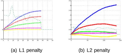
. Results are presented in Fig. 2 with
the mapping coefficients, α
1
i
i {1, 5} in blue, red, green,
cyan and yellow respectively. The convergence criterion,
δ is plotted as the dashed gray line. The results show
the highest coefficient for α
1
1
confirming that signal 1 is
common between the sensors. Applying the L
1
norm penalty
0 5 10 15 20 25 30 35 40 45 50
−0.5
0
0.5
1
1.5
(a) L1 penalty
0 50 100 150
−0.5
0
0.5
1
1.5
2
2.5
3
3.5
(b) L2 penalty
Fig. 2. Results of indirect estimation of Mutual Information for signals
with underlying linear dependency
0 20 40 60 80 100 120 140 160 180 200
−0.2
0
0.2
0.4
0.6
0.8
1
1.2
1.4
1.6
iteration
α
1
/ δ
(a) L1 penalty
0 20 40 60 80 100 120 140 160 180 200
−3
−2
−1
0
1
2
3
4
iteration
α
1
/ δ
(b) L2 penalty
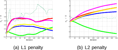
Fig. 3. Results of indirect estimation of MI for non informative signals
to the optimization produced faster convergence, occurring in
iteration 38 compared to 142 iteration with L
2
norm penalty.
It is to be noted that only the non-zero mapping parameter
ideally should be α
1
1
and all others should be zero. However,
due to the approximations in the objective function and the
presence of local minima, the other mapping parameters have
smaller non-zero vales.
Simulation 2: Non Informative Signals
In this simulation signals {1, 2 , 3, 4, 5} are selected as
sensor 1 output and signal {6} is chosen as the sensor 2
output, clearly there is no common signals. Fig. 3 shows that
neither L
1
or L
2
norm penalty has produced convergence
in 200 iterations. In fact the solution based on the L
1
regularization shows a divergence from an optimized solution
verifying there is no common signal.
B. Experiments
Two experiments are performed to evaluate the proposed
method in establishing the relationship between multi-modal
sensory data by identifying informative signals without any
prior knowledge about geometric parameters. Experiment 1:
The purpose is to localise the audio source in the video
data sequence. Experiment 2: The purpose is to identify the
common source in a laser and video data stream.
Experiment 1: Audio and Video Signals: A microphone
and camera were used to capture activity in an office en-
vironment consisting of a person (left on image) reading a
sequence of numbers and another person (right of image)
mimicking unscripted sentences (see Fig. 4(a)). Video data
was captured at 15Hz while audio signal was captured at
48KHz with only 10KHz of content used. Both video and
audio data streams were synchronised in time. Color images
acquired were transformed to grey scale and pixel intensity
values (consisting of 640 480 = 307200 pixels per frame)
of 100 frames were analyzed using raw pixel values. The

Citations
More filters
Posted Content

Arbitrary Talking Face Generation via Attentional Audio-Visual Coherence Learning

TL;DR: A novel arbitrary talking face generation framework is proposed by discovering the audio-visual coherence via the proposed Asymmetric Mutual Information Estimator (AMIE) and a Dynamic Attention (DA) block by selectively focusing the lip area of the input image during the training stage, to further enhance lip synchronization.
Posted Content

High-Resolution Talking Face Generation via Mutual Information Approximation.

TL;DR: A novel high-resolution talking face generation model for arbitrary person is proposed by discovering the cross-modality coherence via Mutual Information Approximation (MIA) by assuming the modality difference between audio and video is larger that of real video and generated video.
Journal ArticleDOI

Forest Sampling Desk Reference

Howard L. Wright
- 01 Jan 2001 - 
Proceedings ArticleDOI

A dependence maximization approach towards street map-based localization

TL;DR: This paper presents a novel approach to 2D street map-based localization for mobile robots that navigate mainly in urban sidewalk environments and employs a computationally efficient estimator of Squared-loss Mutual Information through which it achieved near real-time performance.
Journal ArticleDOI

Dependence maximization localization: a novel approach to 2D street-map-based robot localization

TL;DR: This paper proposes a novel localization approach that can be applied to sidewalks based on existing 2D street maps and employs a computationally efficient estimator of squared-loss mutual information, through which it achieves near real-time performance.
References
More filters
Book ChapterDOI

Hypothesis testing over factorizations for data association

TL;DR: This paper examines the data association problem as the more general hypothesis test between factorizations of a single, learned distribution, and describes an extension of this technique to multisignal association which can be used to determine correspondence while avoiding the computationally prohibitive task of evaluating all hypotheses.

Exploring the Spanish interbank yield curve

TL;DR: In this article, the authors perform an econometric exploration of the Spanish interbank market and estimate a transformation of its yield curve according to a VARMA model based canonical and principal component analysis.
Frequently Asked Questions (15)
Q1. What contributions have the authors mentioned in the paper "Cross-modal localization through mutual information" ?

One possible strategy to address this task is to examine whether the sensor outputs contain information which can be attributed to a common cause. In this paper, the authors present an approach to localise this embedded common information through an indirect method of estimating mutual information between all signal sources. 

Research in several directions to extend the work presented in this paper are currently under way. Combining the indirect estimation methods with direct estimation could couple their respective strengths and would be a fruitful avenue of further research into signal grouping. Constructing a multidimensional feature space by combining the separate features could add value and this would obviously benefit future research outcomes. 

Color images acquired were transformed to grey scale and pixel intensity values (consisting of 640 ∗ 480 = 307200 pixels per frame) of 100 frames were analyzed using raw pixel values. 

Formulating the problem in the feature level rather than signal level will remove the requirement of preserving locality of thedata source. 

Applying the L1 norm penalty to the optimization produced faster convergence, occurring in iteration 72 compared to 110 iteration with L2 norm penalty. 

In order to detect that the optimization has reached a local minima the variation of δ should be contained in a 1.5e−3 limit at least for a minimal convergence span of 5 iterations. 

The maximisation of MI is achieved by maximising the entropies H(Y1) and H(Y2) and minimising the joint entropy, H(Y1, Y2) in (1). 

due to the approximations in the objective function and the presence of local minima, the other mapping parameters have smaller non-zero vales. 

The entropies H(Y1) and H(Y2) can be maximised by selecting the mapping parameters to make the data on the lower dimensional space resemble a uniform distribution. 

the solution of the parameter vectors α1 and α2 should be sparse identifying the minimum number of nonzero elements naturally suggesting the use of the L1 norm as an appropriate penalty function. 

Since the projections α1, α2 may be of very high dimensionality, it is assumed thatmin ‖α1‖1 = |α11 | + |α12 | + · · · |α1n | (16)Therefore the L1 penalty is∂ min ‖α1‖1 ∂Y1(17)further∂|α1| ∂Y11 = ∑n i=1 ∂|α1i | ∂Y11 = ∑ |X−11 |row1 sign|Y11 | ... ∂|α1| ∂Y1i = ∑n i=1 ∂|α1i | ∂Y1i = ∑ |X−11 |rowi sign|Y1i |resulting in∂ min ‖α1‖1 ∂Y1 = ∑ |X−11 | sign|Y1| (18)All iterative optimization methods require stopping criteria to indicate the successful completion of the process. 

joint entropy H(Y1, Y2) can be minimised by selecting the mapping parameters to reflect the joint distribution, (Y1, Y2) is furthest away from a uniform distribution. 

The laser beam of the range finder intersects horizontally at the abdominal area of the standing person capturing the movement of the book. 

They proposed an unsupervised learning method by which the mappings g1(·) and g2(·) can be estimated indirectly, without computing mutual information. 

The L1 norm performs equally well as the L2 norm on overdetermined system of equations while outperforming L2 norm for underdetermined problems [9] especially where the solution is expected to have fewer non zeros than 1/8 of the number of equations.