
All figures (12)

Figure 3. (a) Phase lag Φδz(x0 for different couples of points centered on x0 : δz = 4 px; δz = 8 px; δz = 12 px; δz = 16 px; δz = 32 px, (b) Estimation of the non-dimensioned convection velocity Uc/Uj for the same couples of points centered on x0 
Figure 8. Density field of an underexpanded Mj = 1.56 and ReD = 5× 10 4 jet, obtained by simulation16 
Figure 12. Phase evolution with Strouhal number for different separations between the two sensors monitoring (a) the density field, (b) the gray levels gz in the schlieren images. Separations 2δz/D: 0.121, 0.241, 0.362, 0.482 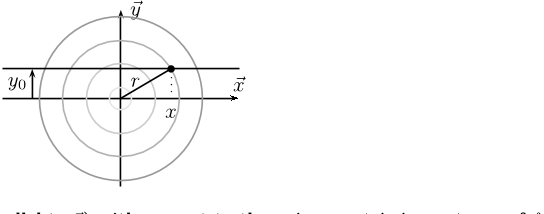
Figure 4. Light beam position (parallel to ~x) with respect to the axisymmetric isocontours of f . 
Figure 11. Radial profiles at axial distance z0/D = 3.8 of the standard deviation for different quantities α normalized by their maximum values; α ≡ density, gy, gz, axial velocity, radial velocity 
Figure 10. Axial evolution of (a) density fluctuations, taken along r/D=0.63 and the line of maximum density fluctuations, (b) the maximum of gray levels gi fluctuations, considering either schlieren images obtained with a knife-edge oriented along the jet axis (gy, ) or normal to the jet axis (gz, ) . The dashed vertical lines correspond to the shock positions. 
Figure 9. Maps of standard deviation of (a) density, (b) the gray level gy in the schlieren image with horizontal knife-edge ( f ≡ ∂ρ ∂y ) , (c) the gray level gz in the schlieren image with vertical knife-edge ( f ≡ ∂ρ ∂z ) . The colorbars in figures (b) and (c) are adjusted so that the maximum value is in white 
Figure 6. Schlieren images obtained from experiments7 at ReD = 2 × 10 6 (left) and from the simulation at ReD = 5× 10 4 (right). 
Figure 7. Synthetic schlieren pictures computed using one 3-D flow density field at a given time t (top), the time-averaged 3-D density field (middle) and the mean density profile combined with equation (5) (bottom). Pictures in the left column correspond to f ≡ ∂ρ/∂y, i.e. (virtual) knife-edge oriented along the jet axis, and pictures in the right column correspond to f ≡ ∂ρ/∂z, i.e. knife-edge normal to the jet axis. Only the top-half of the jet is considered 
Figure 13. Convection velocity evolution with Strouhal number for different separations between the two sensors monitoring (a) the density field, (b) the gray levels gz from schlieren images, (c) the gray levels gy from schlieren images. Separations 2δz/D of 0.121, 0.241, 0.362, 0.482. In figures (b) and (c), the dashed curve corresponds to the result obtained with density signals. 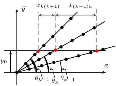
Figure 5. Interpolation method for the computation of ǫf (y0, z0) : the black dots represent the locations where the values of f are known (as a result of the numerical simulation using cylindrical coordinates), the red dots represent the locations where f is interpolated (1-D interpolation in the radial direction at a given θ). Three over the 512 values of θ are represented here. 
Figure 2. Time-averaged density field of an underexpanded, Mj = 1.56 and ReD = 5 × 10 4, jet, obtained by simulation.16 Isovalues of density from 1 to 2.6 kg.m−3, by step 0.2 kg.m−3, are presented.


30 May 2016-