
All figures (10)
 Figure 4: Ice Core Model-Data Comparison at NGRIP: effect of diffusion length (σ) on β. Estimated power spectral density for simulated (purple) vs. observed (black) δ18O of ice and the effect of varying diffusion length parameters. The grey shaded region spans experiments resampling the data 1000 times varying the diffusion length from 12 · σ to 2 · σ. In the case where σ = 0 (the royal blue line, δ18OPRECIP), GCM-simulated data is generally in agreement with the observations.
 Figure 5: Speleothem Calcite Model-Data Comparison: the effect of Karst Transit Time (τ) on β. Simulated vs. Observed δ18O of speleothem calcite at Cascayunga Cave. PSD is plotted, simulated using an ensemble of plausible values (6 months to 5 years) for the karst transit time parameter, τ. The spectrum reddens as the transit time increases. The orange solid line indicates the mean β slope for the observations. Figure illustrates broadening disagreement between simulated and observed speleothem δ18O approaching decadal-centennial timescales.
 Figure 8: Distribution of proxy βI , βD values, GCM+PSM vs. Observed, for the PAGES2k Phase 1 dataset: a. ice cores (blue, left), tree-ring width (green, center), and coral data (orange, right) from PAGES2k (lighter colors) and GCM/PSM (darker colors). (a, b., d., e.): temperature (red), precipitation (dark blue) and PSM ice cores (light blue, right); SPEEDY-IER temperature (red), precipitation (dark blue), and PSM tree-ring width (green, center); and (c., f.): CCSM4 sea-surface temperature (pink), sea-surface salinity (purple), and PSM coral data (orange, right).
 Figure 1: Spectra and β values by proxy type and as a function of timescale. Estimated Power Spectral Density for a purely white noise input climate signal, leaving the effects of the proxy system only. Each PSM was forced with white noise climate input 10,000 times. The median spectrum is shown as the solid line, and shading represents the 95% confidence interval. a. Ice Core δ18O, b. Carbonates (Coral and Speleothem δ18O) c. TRW, Tree Ring Cellulose δ18O.
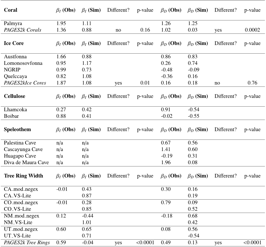 Table 2: βI and βD values for coral, ice core, speleothem, and tree ring cellulose sites, simulated vs. observed for all case studies and the PAGES2k Database. βI is calculated as the mean slope between 2 and 8 years (interannual), and βD is the mean slope between 20 and 200 years (decadal to centennial). Mean PAGES2k vs. PSM simulated overall β values for Coral, Ice Core, and Tree Ring PAGES2k sites with test statistics for difference-of-mean Mann-Whitney/Wilcoxon Rank-Sum tests are given alongside case studies. For TRW, β values were calculated for the four tree ring width sites listed in Table 1, simulated vs. observed, using the Modified Negative Exponential (negex) detrending method and simply calculating the slope after simulating the TRW using the forward model VS-Lite (no detrending). We report difference of means test statistics for the PAGES2k data only, as we have a full distribution of values for these data as opposed to the single-point case studies, where a difference of means test is not appropriate. See SI Table S6 for a comparison of six different detrending methods including RCS, Modified Negative Exponential (negex), Linear, Spline, Hugershoff.
 Figure 2: Coral Aragonite Model-Data Comparison: simulated (pink) and measured (black) spectrum for Palmyra coral data, as well as the effects of altering α2 at Palmyra island alongside the climate inputs to the model (SST, SSS). Straight orange lines are the calculated mean slopes across both decadal to centennial (20-200, βD) and interannual (2-8, βI ) timescales. The black-dotted envelope represents the full range of outcomes given the perturbed salinity parameter space. Low frequency variance observed in the coral data (black dashed line) greatly exceeds that of the simulated pseudo coral data (pink), and the discrepancy grows with increasing timescale. Also shown: simulated sensitivity to salinity changes and potential parameter uncertainties in the PSM (α2), effects on β, (faint black dots), which does not help account for the model-data discrepancies. We removed the mean from all fields prior to computed the PSD.
 Figure 7: Tree-Ring Width Model-Data Comparison: the effect of detrending method on β. For each site, the original measured TRW is plotted in black, along with the PSM (VS-Lite) inputs of temperature (red), precipitation (blue), and the simple VS-Lite generated pseudoproxy data (dark green dashed), which does not include detrending or growth-curve. The negative-exponential detrending method was applied to both the real proxy data and the VS-Lite generated pseudoproxy data (bright green). To estimate reasonable errors for simulated TRW, we took reported errors for the estimated growth parameters in 100 randomized possibilities (grey).
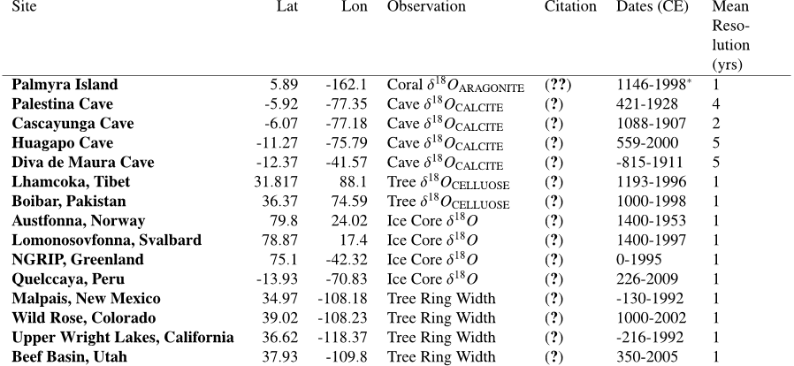 Table 1: List of sites forward modeled and evaluated in this study. By building a workflow connecting paleoclimate proxy data, a climate model, and proxy system models, we evaluate spectral scaling characteristics for five proxy types in four regional case studies. Corals, Ice Cores, Speleothems, Tree-Ring Width, Tree-Ring Cellulose. ∗ Note that the Palmyra coral record is continuous in the interval 1146-1464: we use the previously published, continuous part of the record in this study. This segment has been updated since (?).
 Figure 6: Tree-Ring Cellulose Model-Data Comparison. Estimated Power Spectral Density for Simulated (green) vs. Observed (black) δ18O of tree ring cellulose at (a) Boibar, Pakistan and (b) Lhamcoka, Tibet. We removed the mean from all fields prior to computed the PSD.
 Figure 3: Ice Core Model-Data Comparison. Estimated Power Spectral Density for Simulated vs. Observed δ18O of ice at four sites: (a) NGRIP, (b) Quelccaya, (c) Austfonna, (d) Lomonosovfonna. The PSD for each PSM-generated record is shown (red) alongside climate inputs of temperature (dark blue), precipitation (light blue), and δ18OP (purple). In all cases, the observed ice core record is plotted in black (dashed). Straight orange lines are the calculated mean slopes across both decadal to centennial (20-200, βD) and interannual (2-8, βI ) timescales. Diffusion in the ice core PSM causes higher-than-observed spectral slopes at high frequencies, and may suggest that the simulation of diffusion and compaction is overestimated. PSM-simulated ice cores do not capture the observed higher variance at low-frequencies. We removed the mean from all fields prior to computed the PSD.


