scispace - formally typeset
Search or ask a question
Book ChapterDOI

Multi-label MRF Optimization via a Least Squares s - t Cut

26 Nov 2009-pp 1055-1066
TL;DR: In this article, the k-label Markov random field optimization is approximated by a single binary graph cut, where each vertex in the original graph is replaced by only ceil (log 2 (k )) new vertices and the new edge weights are obtained via a novel least squares solution approximating the original data and label interaction penalties.
Abstract: We approximate the k -label Markov random field optimization by a single binary (s - t ) graph cut. Each vertex in the original graph is replaced by only ceil (log 2 (k )) new vertices and the new edge weights are obtained via a novel least squares solution approximating the original data and label interaction penalties. The s - t cut produces a binary "Gray" encoding that is unambiguously decoded into any of the original k labels. We analyze the properties of the approximation and present quantitative and qualitative image segmentation results, one of the several computer vision applications of multi label-MRF optimization.

Summary (3 min read)

1. Introduction

  • A solid oxide fuel cell has an advantage of high power generation efficiency even in systems with a relatively small capacity.
  • Steam is electrochemically decomposed into hydrogen and oxygen while consuming electrical energy.
  • They observed a decrease in the discharge capacity but nearly 40% of the storage metal remained active even after 10,000 cycles.
  • Because this new battery is still its early stage of the development, the authors assume one of the simplest configurations of the SOIAB systems to clarify the most fundamental characteristics of the system.
  • The analyzed system is based on 0-D models of the constituent components such as the SOEC, redox metal reactor and heat exchangers introduced in their previous study [35].

2. Numerical modeling

  • 1. Outline of the system Figure 1 (a) schematically shows one of the simplest configurations of the SOIAB and its concept.
  • The authors need to introduce two blowers in this configuration.
  • The SOEC functions in an electrolysis mode.
  • (1) O2- migrates in the electrolyte to the air electrode, where oxygen is released to the air flow.
  • Fe3O4 in the Fe box is reduced by hydrogen and the resultant steam-rich mixture gas is recirculated to the fuel electrode for further electrolysis by the fuel-blower.

2.2. Assumptions and conditions

  • Because the simulation method is basically the same as the one the authors developed in their previous study, it is only briefly explained in this section.
  • Effective thermal insulation will be important in order to realize the system at an allowable size and cost.
  • The operating temperatures of the SOEC and the Fe box are assumed to be the same for simplicity and set at 600 oC.
  • The average current densities during charge/discharge processes are 50 mA/cm2 and 100 mA/cm2, respectively.
  • The effects of the operation conditions are discussed in sections 3.2- 3.4.

2.3. System round-trip efficiency

  • Considering the thermal energy input to the system, the authors define the system round-trip efficiency, η, as DCC D QQP Pη ++ = . (9) where PC and PD are the input and output electricity.
  • QC and QD are the heat inputs to the system during the charge and discharge processes, respectively.
  • In the calculation of the system round-trip efficiency, QC and QD are allowed to take non-negative values.
  • If there is excess heat generation in the system, the authors assume that the excess heat is exhausted to the atmosphere and QC or QD is set to zero when calculating the system round-trip efficiency.

2.4. Generation/absorption of thermal energy and heat transfer

  • In Fig. 1, the main heat input/output during the operations are shown with the red, blue and yellow arrows.
  • The authors first explain the heat input/output assuming the simple system shown in Fig. 1 (a) and then the system with thermal recirculation shown in Fig. 1 (b) is explained at the last of this section.
  • The total heat input during the charge and discharge operation, QC and QD, respectively, are obtained by summing all the terms related to the heat input/output except for the heat generated by the losses in the SOEC.
  • The reduction of Qair and Qfuel is effective for enhancing the system round-trip efficiency.

3.1. Energy budget of fundamental system with/without thermal recirculation

  • To clarify fundamental characteristics of the SOIAB, the authors start with a preliminary discussion of a simple system and stepwisely take more realistic factors into account.
  • If the authors consider the thermal input, however, the round-trip efficiency of this ideal system is evaluated to be 73% from Eq. (9).
  • For this case, a Sankey diagram is shown in Fig. 2 (a), which shows the energy flow in the system.
  • Since the thermal energy input to preheat the gases is markedly less than that shown in Fig. 2 (b), the reaction heat in the charge process becomes the main component of the heat input.
  • Considering the heat-loss penalty of a small-scale regenerator, however, the use of a regenerator will be more suitable for large-scale systems.

3.2. Effects of heat exchanger effectiveness on round-trip efficiency

  • Figure 3 shows the effects of the heat exchanger effectiveness on the system round-trip efficiency.
  • This is reasonable because the amount of heat exchanged by HEX3 is the largest among the three heat exchangers.
  • At the point marked with a square, which is “a heat-balanced point”, the input heat during the discharge process, QD, is equal to zero.
  • The effectiveness of HEX1 also substantially affects the round-trip efficiency.
  • The line comes to an end at a point marked “x” in this case.

3.3. Effects of gas utilization factors on round-trip efficiency and efficient and

  • The effects of the gas utilization factors are shown in Fig.
  • Because the air flow rate is generally higher than the fuel flow rate, the effect of the air utilization factor on the round-trip efficiency is more prominent.
  • To observe the effects of the gas utilization factors within the limitation of the 0-D model simulation, the authors calculate the EMF at the SOEC exit, Eout, for each combination of fuel and air utilization factors, which is normalized by the EMF at the inlet, Ein, and is shown in Fig. 4 (b) as black contour lines.
  • On the other hand, the red line in Fig. 4 (b) indicates the limit at which the fuel-blower temperature reaches its maximum allowable value of 150 oC; the system must be operated in the region to the left of the red line in the figure.
  • The acute-angled region bounded by the blue and red lines in Fig. 4 (b) shows conditions for efficient and uniform operation under the constraints set in this study.

3.4. Effects of current density on round-trip efficiency

  • As shown in Fig. 5, the round-trip efficiency changes with the current density during the charge or discharge operation.
  • Again, note that the operation time changes with the current density according to the relationship tC iC = tD iD.
  • If the current density in the charge operation is low, the required heat transfer surface area of the HEXs decreases owing to the low flow rates.
  • This results in an insufficient heat recovery for the preheating of air during the discharge operation.
  • The demand for additional heat input during the discharge operation increases, lowering the round-trip efficiency.

4. Conclusions

  • A system simulation model of an SOIAB system was developed to investigate the fundamental characteristics during the charge and discharge operations.
  • The system round-trip efficiency can be recovered by introducing heat exchangers to circulate thermal energy from the exhaust gases.
  • (2) The effects of the heat exchanger effectiveness, gas utilization and current density were examined.
  • The system round-trip efficiency considerably drops under these operation conditions.
  • This constraint gives a lower limit for the air utilization factor.

Did you find this useful? Give us your feedback

Figures (8)

Content maybe subject to copyright    Report

Multi-label MRF Optimization
via a Least Squares s t Cut
Ghassan Hamarneh
School of Computing Science, Simon Fraser University, Canada
Abstract. We approximate the k-label Markov random field optimiza-
tion by a single binary (st) graph cut. Each vertex in the original graph
is replaced by only ceil(log
2
(k)) new vertices and the new edge weights
are obtained via a novel least squares solution approximating the origi-
nal data and label interaction penalties. The s t cut produces a binary
“Gray” encoding that is unambiguously decoded into any of the original
k labels. We analyze the properties of the approximation and present
quantitative and qualitative image segmentation results, one of the sev-
eral computer vision applications of multi label-MRF optimization.
1 Introduction
Many visual computing tasks can be formulated as graph labeling problems,
e.g. segmentation and stereo-reconstruction [1], in which one out of k labels is
assigned to each graph vertex. This may be formulated as a k-way cut problem:
Given graph G(V,E)with|V | vertices v
j
V and |E| edges e
v
i
,v
j
= e
ij
E
V × V with weights w(e
ij
)=w
ij
> 0, find an optimal k-cut C
E with min-
imal cost |C
| = argmin
C
|C|,where|C| =
e
ij
C
w
ij
, such that E\C breaks
the graph into k groups of labelled vertices. This k-cut formulation encodes the
semantics of the problem at hand (e.g. segmentation) into w
ij
. However, if the
optimal label assigned to a vertex depends on the labels assigned to other vertices
(e.g. to regularize the label field), setting w
ij
i, j becomes less straightforward.
The Markov random field (MRF) formulation captures this desired label inter-
action via an energy ξ(l) to be minimized with respect to the vertex labels l.
ξ(l)=
v
i
V
D
i
(l
i
)+λ
(v
i
,v
j
)E
V
ij
(l
i
,l
j
,d
i
,d
j
)(1)
where D
i
(l
i
) penalizes labeling v
i
with l
i
,andV
ij
, aka prior, penalizes assigning
labels (l
i
,l
j
) to neighboring vertices
1
. V
ij
may be influenced by the data value
d
i
at v
i
(e.g. image intensity). λ controls the relative importance of D
i
and V
ij
.
For labeling a P -pixel image, typically a graph G is constructed with |V | = P .
To encode D
i
(l
i
), G may be augmented with k new terminal vertices {t
j
}
k
j=1
;
each representing one of the k labels (Figure 2(a)) and w
v
i
,t
j
set inversely pro-
portional to D
i
(l
j
). When V
ij
= V
ij
(d
i
,d
j
), i.e. independent of l
i
and l
j
, V
ij
may be encoded by w
v
i
,v
j
V
ij
(d
i
,d
j
). The random walker [2] globally solves a
1
Higher order priors, e.g. 3
rd
order V
ijk
(l
i
,l
j
,l
k
), are also possible.
G. Bebis et al. (Eds.): ISVC 2009, Part I, LNCS 5875, pp. 1055–1066, 2009.
c
Springer-Verlag Berlin Heidelberg 2009

1056 G. Hamarneh
labeling problem of this type, i.e. disregarding label interaction. Solving multi-
label MRF optimization for any interaction penalty remains an active research
area. In [3], the globally optimal binary (k=2) labeling is found using min-cut
max-flow. For k>2 with convex prior, the global minimizer is attained by
replacing each single k-label variable with k [4] or by using k 1 [5] boolean
variables. However, convex priors tend to over-smooth the label field. For k>2
with metric or semi-metric priors, Boykov et al. performed range moves using
binary cuts to expand or swap labels [1]. Other range moves were proposed in
[6,7]. More recent approaches to multi-label MRF optimization were proposed
based on linear programming relaxation using primal-dual [8], message passing
or belief propagation [9], and partial optimality [10] (see [11] for a recent survey).
In this paper, we focus on optimal encoding of the k-label MRF energy solely
into the edge weights of a graph. We impose no restrictions on k, or on the order
(2
nd
or higher) or type (e.g. non-convex, non-metric, or spatially varying) of the
label interaction penalty. The calculated edge weights are optimal in the sense
that they minimize the least squares (LS) error when solving a linear system of
equations capturing the original MRF penalties. Further, we transform the multi-
labelling problem to a binary st cut, in which each vertex in the original graph is
replaced by the most compact boolean representation; only ceil(log
2
(k)) vertices
represent each k-label variable. In [12], a general framework for converting multi-
label problems to binary ones is presented. In contrast to our work, [12] solved a
system of equations to find the boolean encoding function (not the edge weights),
they did not use LS, and their resulting binary problem can still include label
interaction. We perform a single (non-iterative and initialization-independent)
s t cut to obtain a “Gray” binary encoding, which is then unambiguously
decoded into the k labels. Besides its optimality features, LS enables offline pre-
computation of pseudoinverse matrices that can be re-used for different graphs.
2Method
2.1 Reformulating the Multi-label MRF as an s t Cut
Given a graph G(V,E), the objective is to label each vertex v
i
V with a label
l
i
∈L
k
= {l
0
,l
1
, ..., l
k1
}. Rather than labeling v
i
with l
i
∈L
k
, we replace v
i
with b vertices (v
ij
)
b
j=1
, and binary-label them with (l
ij
)
b
j=1
, i.e. l
ij
∈L
2
=
{l
0
,l
1
}. b is chosen such that 2
b
k or b = ceil(log
2
(k)), i.e. alongenough
sequence of bits to be decoded into l
i
∈L
k
2
. To this end, we transform G(V,E)
into a new graph G
2
(V
2
,E
2
) with additional source s and sink t nodes, i.e.|V
2
| =
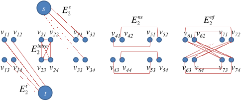
b|V | +2. E
2
includes terminal links E
tlinks
2
= E
t
2
E
s
2
where |E
t
2
| = |E
s
2
| = |V
2
|;
neighborhood links E
nlinks
2
= E
ns
2
E
nf
2
where |E
nlinks
2
| = b
2
|E|, |E
ns
2
| = b|E|,
and |E
nf
2
| =(b
2
b)|E|; and intra-links E
intra
2
where |E
intra
2
| =
b
2
|V |.Figure
1 shows these different types of edges. Following an s t cut on G
2
, vertices v
ij
that remain connected to s are assigned label 0, and the remaining are connected
2
We distinguish between the decimal (base 10) and binary (base 2) encoding of the
labels using the notation (l
i
)
10
and (l
i
)
2
=(l
i1
,l
i2
, ··· ,l
ib
)
2
, respectively.

Multi-label MRF Optimization via a Least Squares s t Cut 1057
t
s
v
21
v
22
v
23
v
24
v
11
v
12
v
13
v
14
v
41
v
42
v
43
v
44
v
31
v
32
v
33
v
34
v
51
v
52
v
53
v
54
E
2
t
E
2
s
E
2
intra
E
2
ns
v
61
v
62
v
63
v
64
v
71
v
72
v
73
v
74
E
2
nf
Fig. 1. Edge types in the s t graph. Shown are seven groups of vertex quadruplets,
b=4, and only sample edges from E
t
2
,E
s
2
,E
ns
2
,E
nf
2
, and E
intra
2
.
t
s
t
0
t
1
t
2
t
3
v
1
v
2
v
3
v
4
v
5
v
21
v
22
v
31
v
32
v
41
v
42
v
51
v
52
l
0
l
1
l
2
l
3
v
1
v
2
v
3
v
4
v
5
00
01 10
11
v
11
v
12
(a)
(b)
(c)
l
0
l
1
l
2
l
3
Fig. 2. Reformulating the multi-label problem as an s t cut. (a) Labeling vertices
{v
i
}
5
i=1
with labels {l
j
}
3
j=0
(only t-links are shown). (b) New graph with 2 terminal
nodes {s, t}, b =2newvertices(v
i1
and v
i2
inside the dashed circles) replacing each
v
i
in (a), and 2 terminal edges for each v
ij
.Ans t cut on (b) is depicted as the green
curve. (c) Labeling v
i
in (a) is based on the s t cut in (b): Pairs of (v
i1
,v
i2
) assigned
to (s, s) are labeled with binary string 00, (s, t) with 01, (t, s) with 10, and (t, t)with
11. The binary encodings {00,01,10,11} in turn reflect the original 4 labels {l
j
}
3
j=0
.
to t and assigned label 1. The string of b binary labels l
ij
∈L
2
assigned to v
ij
are
then decoded back into a decimal number indicating the label l
i
∈L
k
assigned
to v
i
(Figure 2).
It is important to set the edge weights of E
2
in such a way that decoding the
binary labels resulting from the s t cut of G
2
results in optimal (or close to
optimal) labels for the original multi-label problem. To achieve this, we derive a
system of linear equations capturing the relation between the original multi-label
MRF penalties and the s t cut cost incurred when generating different label
configurations. We then calculate the weights of E
2
as the LS error solution to
these equations. The next sections expose the details.
2.2 Data Term Penalty: Severing T-Links and Intra-Links
The 1
st
order penalty D
i
(l
i
) in (1) is the cost of assigning l
i
to v
i
in G,which
entails assigning a corresponding sequence of binary labels (l
ij
)
b
j=1
to (v
ij
)
b
j=1
in G
2
. To assign (l
i
)
2
toastringofb vertices, appropriate terminal links must
be cut. To assign a 0 (resp. 1) label to v
ij
, the edge connecting v
ij
to t (resp.

1058 G. Hamarneh
11
01
10
00
100100
11
t
s
t
s
t
s
t
s
t
s
t
s
t
s
t
s
000 001 010 011 100 101 110 111
s
t
s
t
s
t
s
t
s
t
Fig. 3. The 2
b
ways of cutting through {v
ij
}
b
j=1
for b = 2 (left) and b = 3 (right) with
the resulting binary codes {00, 01, 10, 11} and {000, 001, ··· , 111}
s) must be severed (Figure 3). Therefore, the cost of severing t-links in G
2
to
assign l
i
to vertex v
i
in G is calculated as
D
tlinks
i
(l
i
)=
b
j=1
l
ij
w
v
ij
,s
+
¯
l
ij
w
v
ij
,t
(2)
where
¯
l
ij
denotes the unary complement (NOT) of l
ij
.TheG
2
s t cut severing
the t-links, as per (2), will also result in severing edges in E
intra
2
(Figure 1). In
particular, e
im,in
E
intra
2
will be severed iff the st cut leaves v
im
connected to
one terminal, say s (resp. t), while v
in
remains connected to the other terminal
t (resp. s). If this condition holds, then w
v
im
,v
in
will contribute to the cost.
Therefore, the cost of severing intra-links in G
2
to assign l
i
to vertex v
i
in G is
D
intra
i
(l
i
)=
b
m=1
b
n=m+1
(l
im
l
in
) w
v
im
,v
in
(3)
where denotes binary XOR. The total data penalty is the sum of (2) and (3),
D
i
(l
i
)=D
tlinks
i
(l
i
)+D
intra
i
(l
i
). (4)
2.3 Prior Term Penalty: Severing N-Links
The interaction penalty V
ij
(l
i
,l
j
,d
i
,d
j
) for assigning l
i
to v
i
and l
j
to neighboring
v
j
in G must equal the cost of assigning a sequence of binary labels (l
im
)
b
m=1
to
(v
im
)
b
m=1
and (l
jn
)
b
n=1
to (v
in
)
b
n=1
in G
2
. The cost of this cut can be calculated
as (Figure 4)
V
ij
(l
i
,l
j
,d
i
,d
j
)=
b
m=1
b
n=1
(l
im
l
jn
) w
v
im
,v
jn
. (5)
This effectively adds the edge weight between v
im
and v
jn
to the cut cost iff the
cut results in one vertex of the edge connected to one terminal (s or t) while
the other vertex connected to the other terminal (t or s). Note that we impose
no restrictions on the left hand side of (5), e.g. it could reflect non-convex or
non-metric priors, spatially-varying, or even higher order label interaction.

Multi-label MRF Optimization via a Least Squares s t Cut 1059
v
i
v
j
v
i
v
j
v
i1
v
j1
v
i2
v
j2
v
i3
v
j3
v
i1
v
j1
v
i2
v
j2
00 00
000 000
01 10 11 10 11 11
011 100 111 110
Fig. 4. Severing n-links between neighboring vertices v
i
and v
j
for b = 2 (four examples
are shown in the top row) and b = 3 (three examples in the bottom row). The cut is
depicted as a red curve. In the last two examples for b = 3, the colored vertices are
translated while maintaining the n-links in order to clearly show that the severed n-links
for each case follow (5).
2.4 Edge Weight Approximation with Least Squares
Equations (4) and (5) dictate the relationship between the penalty terms (D
i
and V
ij
) of the original multi-label problem and the severed edge weights w
ij,mn
;
e
ij,mn
E
2
of the s t graph G
2
. What remains missing before applying the
s t cut, however, is to find these edge weights.
Edge weights of t-links and intra-links. For b =1(i.e. binary labelling),
(3) simplifies to D
intra
i
(l
i
) = 0 and (4) simplifies to D
i
(l
i
)=l
i1
w
v
i1
,s
+
¯
l
i1
w
v
i1
,t
.
With l
i
= l
i1
for b = 1, substituting the two possible values for l
i
= {l
0
,l
1
},we
obtain
l
i
= l
0
D
i
(l
0
)=l
0
w
v
i1
,s
+
¯
l
0
w
v
i1
,t
=0w
v
i1
,s
+1w
v
i1
,t
l
i
= l
1
D
i
(l
1
)=l
1
w
v
i1
,s
+
¯
l
1
w
v
i1
,t
=1w
v
i1
,s
+0w
v
i1
,t
(6)
which can be written in matrix form A
1
X
i
1
= B
i
1
as
01
10
w
v
i1
,s
w
v
i1
,t
=
D
i
(l
0
)
D
i
(l
1
)
where X
i
1
is the vector of unknown edge weights connecting vertex v
i1
to s and t,
B
i
1
is the data penalty for v
i
,andA
1
is the matrix of coefficients. The subscript
1inA
1
,X
i
1
, and B
i
1
indicates that this matrix equation is for b = 1. Clearly, the
solution is trivial and expected: w
v
i1
,s
= D
i
(l
1
)andw
v
i1
,t
= D
i
(l
0
)
For b = 2, we address multi-label problems of k = {3, 4},or2
b1
=2<k
2
b
= 4 labels. Substituting the 2
b
= 4 possible label values, ((0,0),(0,1),(1,0),
and (1,1)), of (l
i
)
2
=(l
i1
,l
i2
) in (4) we obtain
(0, 0) D
i
(l
0
)=0w
v
i1
,s
+1w
v
i1
,t
+0w
v
i2
,s
+1w
v
i2
,t
+0w
v
i1
,v
i2
(0, 1) D
i
(l
1
)=0w
v
i1
,s
+1w
v
i1
,t
+1w
v
i2
,s
+0w
v
i2
,t
+1w
v
i1
,v
i2
(1, 0) D
i
(l
2
)=1w
v
i1
,s
+0w
v
i1
,t
+0w
v
i2
,s
+1w
v
i2
,t
+1w
v
i1
,v
i2
(1, 1) D
i
(l
3
)=1w
v
i1
,s
+0w
v
i1
,t
+1w
v
i2
,s
+0w
v
i2
,t
+0w
v
i1
,v
i2
(7)
which can be written in matrix form A
2
X
i
2
= B
i
2
as

Citations
More filters
Journal ArticleDOI
TL;DR: This paper augments the level set framework with the ability to handle these two intuitive geometric relationships, containment and exclusion, along with a distance constraint between boundaries of multi-region objects, and compared this framework with its counterpart methods in the discrete domain.
Abstract: Incorporating prior knowledge into image segmentation algorithms has proven useful for obtaining more accurate and plausible results. Two important constraints, containment and exclusion of regions, have gained attention in recent years mainly due to their descriptive power. In this paper, we augment the level set framework with the ability to handle these two intuitive geometric relationships, containment and exclusion, along with a distance constraint between boundaries of multi-region objects. Level set's important property of automatically handling topological changes of evolving contours/surfaces enables us to segment spatially-recurring objects (e.g., multiple instances of multi-region cells in a large microscopy image) while satisfying the two aforementioned constraints. In addition, the level set approach gives us a very simple and natural way to compute the distance between contours/surfaces and impose constraints on it. The downside, however, is a local optimization framework in which the final segmentation solution depends on the initialization. In fact, here, we sacrifice the optimizability (local instead of global solution) in exchange for lower space complexity (less memory usage) and faster runtime (especially for large microscopic images) as well as no grid artifacts. Nevertheless, the result from validating our method on several biomedical applications showed the utility and advantages of this augmented level set framework (even with rough initialization that is distant from the desired boundaries). We also compared our framework with its counterpart methods in the discrete domain and reported the pros and cons of each of these methods in terms of metrication error and efficiency in memory usage and runtime.

25 citations

Proceedings ArticleDOI
20 Jun 2011
TL;DR: All possible ways of building graphs and the associated energies minimized, leading to the exhaustive family of energies minimizable exactly by a graph cut are studied, including energies that do not satisfy the submodularity condition.
Abstract: Graph cuts are widely used in many fields of computer vision in order to minimize in small polynomial time complexity certain classes of energies. These specific classes depend on the way chosen to build the graphs representing the problems to solve. We study here all possible ways of building graphs and the associated energies minimized, leading to the exhaustive family of energies minimizable exactly by a graph cut. To do this, we consider the issue of coding pixel labels as states of the graph, i.e. the choice of state interpretations. The family obtained comprises many new classes, in particular energies that do not satisfy the submodularity condition, including energies that are even not permuted-submodular. A generating subfamily is studied in details, in particular we propose a canonical form to represent Markov random fields, which proves useful to recognize energies in this subfamily in linear complexity almost surely, and then to build the associated graph in quasilinear time. A few experiments are performed, to illustrate the new possibilities offered.

6 citations

References
More filters
Book
01 Jan 1991
TL;DR: This book gives a thorough, up-to-date treatment of the behavior of numerical algorithms in finite precision arithmetic by combining algorithmic derivations, perturbation theory, and rounding error analysis.
Abstract: From the Publisher: What is the most accurate way to sum floating point numbers? What are the advantages of IEEE arithmetic? How accurate is Gaussian elimination and what were the key breakthroughs in the development of error analysis for the method? The answers to these and many related questions are included here. This book gives a thorough, up-to-date treatment of the behavior of numerical algorithms in finite precision arithmetic. It combines algorithmic derivations, perturbation theory, and rounding error analysis. Software practicalities are emphasized throughout, with particular reference to LAPACK and MATLAB. The best available error bounds, some of them new, are presented in a unified format with a minimum of jargon. Because of its central role in revealing problem sensitivity and providing error bounds, perturbation theory is treated in detail. Historical perspective and insight are given, with particular reference to the fundamental work of Wilkinson and Turing, and the many quotations provide further information in an accessible format. The book is unique in that algorithmic developments and motivations are given succinctly and implementation details minimized, so that attention can be concentrated on accuracy and stability results. Here, in one place and in a unified notation, is error analysis for most of the standard algorithms in matrix computations. Not since Wilkinson's Rounding Errors in Algebraic Processes (1963) and The Algebraic Eigenvalue Problem (1965) has any volume treated this subject in such depth. A number of topics are treated that are not usually covered in numerical analysis textbooks, including floating point summation, block LU factorization, condition number estimation, the Sylvester equation, powers of matrices, finite precision behavior of stationary iterative methods, Vandermonde systems, and fast matrix multiplication. Although not designed specifically as a textbook, this volume is a suitable reference for an advanced course, and could be used by instructors at all levels as a supplementary text from which to draw examples, historical perspective, statements of results, and exercises (many of which have never before appeared in textbooks). The book is designed to be a comprehensive reference and its bibliography contains more than 1100 references from the research literature. Audience Specialists in numerical analysis as well as computational scientists and engineers concerned about the accuracy of their results will benefit from this book. Much of the book can be understood with only a basic grounding in numerical analysis and linear algebra. About the Author Nicholas J. Higham is a Professor of Applied Mathematics at the University of Manchester, England. He is the author of more than 40 publications and is a member of the editorial boards of the SIAM Journal on Matrix Analysis and Applications and the IMA Journal of Numerical Analysis. His book Handbook of Writing for the Mathematical Sciences was published by SIAM in 1993.

1,911 citations

Journal ArticleDOI
TL;DR: An alternative method based on the preflow concept of Karzanov, which runs as fast as any other known method on dense graphs, achieving an O(n) time bound on an n-vertex graph and faster on graphs of moderate density.
Abstract: All previously known efficient maximum-flow algorithms work by finding augmenting paths, either one path at a time (as in the original Ford and Fulkerson algorithm) or all shortest-length augmenting paths at once (using the layered network approach of Dinic). An alternative method based on the preflow concept of Karzanov is introduced. A preflow is like a flow, except that the total amount flowing into a vertex is allowed to exceed the total amount flowing out. The method maintains a preflow in the original network and pushes local flow excess toward the sink along what are estimated to be shortest paths. The algorithm and its analysis are simple and intuitive, yet the algorithm runs as fast as any other known method on dense graphs, achieving an O(n3) time bound on an n-vertex graph. By incorporating the dynamic tree data structure of Sleator and Tarjan, we obtain a version of the algorithm running in O(nm log(n2/m)) time on an n-vertex, m-edge graph. This is as fast as any known method for any graph density and faster on graphs of moderate density. The algorithm also admits efficient distributed and parallel implementations. A parallel implementation running in O(n2log n) time using n processors and O(m) space is obtained. This time bound matches that of the Shiloach-Vishkin algorithm, which also uses n processors but requires O(n2) space.

1,700 citations

Journal ArticleDOI
TL;DR: A novel graph theoretic approach for data clustering is presented and its application to the image segmentation problem is demonstrated, resulting in an optimal solution equivalent to that obtained by partitioning the complete equivalent tree and is able to handle very large graphs with several hundred thousand vertices.
Abstract: A novel graph theoretic approach for data clustering is presented and its application to the image segmentation problem is demonstrated. The data to be clustered are represented by an undirected adjacency graph G with arc capacities assigned to reflect the similarity between the linked vertices. Clustering is achieved by removing arcs of G to form mutually exclusive subgraphs such that the largest inter-subgraph maximum flow is minimized. For graphs of moderate size ( approximately 2000 vertices), the optimal solution is obtained through partitioning a flow and cut equivalent tree of G, which can be efficiently constructed using the Gomory-Hu algorithm (1961). However for larger graphs this approach is impractical. New theorems for subgraph condensation are derived and are then used to develop a fast algorithm which hierarchically constructs and partitions a partially equivalent tree of much reduced size. This algorithm results in an optimal solution equivalent to that obtained by partitioning the complete equivalent tree and is able to handle very large graphs with several hundred thousand vertices. The new clustering algorithm is applied to the image segmentation problem. The segmentation is achieved by effectively searching for closed contours of edge elements (equivalent to minimum cuts in G), which consist mostly of strong edges, while rejecting contours containing isolated strong edges. This method is able to accurately locate region boundaries and at the same time guarantees the formation of closed edge contours. >

1,223 citations

Journal ArticleDOI
TL;DR: The sequential tree-reweighted message passing (STE-TRW) algorithm as discussed by the authors is a modification of Tree-Reweighted Maximum Product Message Passing (TRW), which was proposed by Wainwright et al.
Abstract: Algorithms for discrete energy minimization are of fundamental importance in computer vision. In this paper, we focus on the recent technique proposed by Wainwright et al. (Nov. 2005)- tree-reweighted max-product message passing (TRW). It was inspired by the problem of maximizing a lower bound on the energy. However, the algorithm is not guaranteed to increase this bound - it may actually go down. In addition, TRW does not always converge. We develop a modification of this algorithm which we call sequential tree-reweighted message passing. Its main property is that the bound is guaranteed not to decrease. We also give a weak tree agreement condition which characterizes local maxima of the bound with respect to TRW algorithms. We prove that our algorithm has a limit point that achieves weak tree agreement. Finally, we show that, our algorithm requires half as much memory as traditional message passing approaches. Experimental results demonstrate that on certain synthetic and real problems, our algorithm outperforms both the ordinary belief propagation and tree-reweighted algorithm in (M. J. Wainwright, et al., Nov. 2005). In addition, on stereo problems with Potts interactions, we obtain a lower energy than graph cuts

1,116 citations

Frequently Asked Questions (16)
Q1. What contributions have the authors mentioned in the paper "Multi-label mrf optimization via a least squares s − t cut" ?

The authors analyze the properties of the approximation and present quantitative and qualitative image segmentation results, one of the several computer vision applications of multi label-MRF optimization. 

More elaborate analysis of the algorithm ( e. g. error bounds, value of the minimized energy, computational complexity, running times ) and comparison with state-of-the-art approaches on standard benchmarks is left for future work. 

The LS error in edge weights induces error in the s − t cut or binary labeling, which is decoded into a suboptimal solution to the multi-label problem. 

Many visual computing tasks can be formulated as graph labeling problems, e.g. segmentation and stereo-reconstruction [1], in which one out of k labels is assigned to each graph vertex. 

The authors perform a single (non-iterative and initialization-independent) s − t cut to obtain a “Gray” binary encoding, which is then unambiguously decoded into the k labels. 

the cost of severing intra-links in G2 to assign li to vertex vi in G isDintrai (li) =b∑m=1b∑n=m+1(lim ⊕ lin) wvim,vin (3)where ⊕ denotes binary XOR. 

every sequence of b binary labels (vij)bj=1 is decoded to a decimal label li ∈ Lk = {l0, l1, ..., lk−1}, ∀vi ∈ V , i.e. the solution to the original multi-label MRF problem. 

The authors then construct GLSE , a noisy version of G, by adding uniformly distributed noise with support [0, noise level] to the edge weights. 

the authors are exploring the use of non-negative least squares (e.g. Chapter 23 in [16]) to guarantee non-negative edge weights as well as quantifying the benefits of the Gray encoding. 

The Markov random field (MRF) formulation captures this desired label interaction via an energy ξ(l) to be minimized with respect to the vertex labels l.ξ(l) = ∑vi∈V Di(li) + λ∑(vi,vj)∈E Vij(li, lj , di, dj) (1)where Di(li) penalizes labeling vi with li, and Vij , aka prior, penalizes assigning labels (li, lj) to neighboring vertices1. 

If Vij(li, lj , di, dj) = Vij(di, dj), i.e. label-independent, the authors can simply ignore the outcome of li ⊕ lj by setting it to a constant. 

The calculated edge weights are optimal in the sense that they minimize the least squares (LS) error when solving a linear system of equations capturing the original MRF penalties. 

(4)The interaction penalty Vij(li, lj, di, dj) for assigning li to vi and lj to neighboring vj in G must equal the cost of assigning a sequence of binary labels (lim)bm=1 to (vim)bm=1 and (ljn) b n=1 to (vin) b n=1 in G2. 

the cost of severing t-links in G2 to assign li to vertex vi in G is calculated asDtlinksi (li) =b∑j=1lijwvij ,s + l̄ijwvij ,t (2)where l̄ij denotes the unary complement (NOT) of lij . 

For b = 2, (5) simplifies toVij(li, lj , di, dj) = (li1 ⊕ lj1)wvi1,vj1 + (li1 ⊕ lj2)wvi1,vj2+ (li2 ⊕ lj1)wvi2,vj1 + (li2 ⊕ lj2)wvi2,vj2 (15)The authors can now substitute all possible 2b2b = 22b = 16 combinations of the pairs of interacting labels (li, lj)∈{l0, l1, l2, l3}×{l0, l1, l2, l3}, or equivalently, ((li)2, (lj)2) ∈ {00, 01, 10, 11}× {00, 01, 10, 11}. 

in the general case when Vij depends on the labels li and lj of the neighboring vertices vi and vj , a single edge weight is insufficient to capture such elaborate label interactions, intuitively, because wi,j needs to take on a different value for every pair of labels.