scispace - formally typeset
Search or ask a question
Journal ArticleDOI

Producing the tangency portfolio as a corner portfolio

01 Jul 2013-Rairo-operations Research (EDP Sciences)-Vol. 47, Iss: 3, pp 311-320
TL;DR: This paper introduces a method for which the tangency portfolio can be produced as a corner portfolio and shows that how this method can be used for tracing out the M-V efficient frontier when problem contains a riskless asset in which the borrowing is not allowed.
Abstract: One-fund theorem states that an efficient portfolio in a Mean-Variance (M-V) portfolio selection problem for a set of some risky assets and a riskless asset can be represented by a combination of a unique risky fund (tangency portfolio) and the riskless asset In this paper, we introduce a method for which the tangency portfolio can be produced as a corner portfolio So, the tangency portfolio can be computed easily and fast by any algorithm designed for tracing out the M-V efficient frontier via computing the corner portfolios Moreover, we show that how this method can be used for tracing out the M-V efficient frontier when problem contains a riskless asset in which the borrowing is not allowed

Summary (2 min read)

1. Introduction

  • The aim of classic Mean-Variance (M-V) portfolio optimization, originated from the seminal work of Markowitz [7], is to maximize the expected return of a portfolio and minimize its variance as the measure of risk.
  • The optimal CAL has the highest possible slop and is tangent to the efficient frontier of risky assets.
  • Niedermayer and Niedermayer [13] provide a Matlab quadratic optimization tool based on Markowitz’s CLA.
  • The authors present an algorithm, based on Tütüncü’s results, for which the tangency portfolio can be produced as a corner portfolio.

2. The tangency portfolio

  • Rn, where each xi is the weight allocated to the ith asset.
  • Since variance is strictly convex, x∗ is unique.
  • Let ρmin be the expected return of the Global Minimum-Variance (GMV) portfolio which has the minimum variance between all feasible portfolios.
  • See Theorem 1 of [17] and the paragraph following the theorem.
  • The assertions of Theorem 2.3 are presented with respect to corresponding Lagrangian multiplier of any optimal portfolio.

3. The modified problem

  • The authors introduce the modified problem that corresponds to Problem 1, which contains an additional variable xf so-called free variable.
  • (The value of c can be interpreted as the variance of the return of the asset xf which its return is uncorrelated with the returns of the other assets and has the expected value rf ).
  • Obviously x satisfies the conditions of Problem 1, if and only if, (x, 0) satisfies the conditions of Problem 2.
  • Then the following theorem holds: Theorem 3.2.
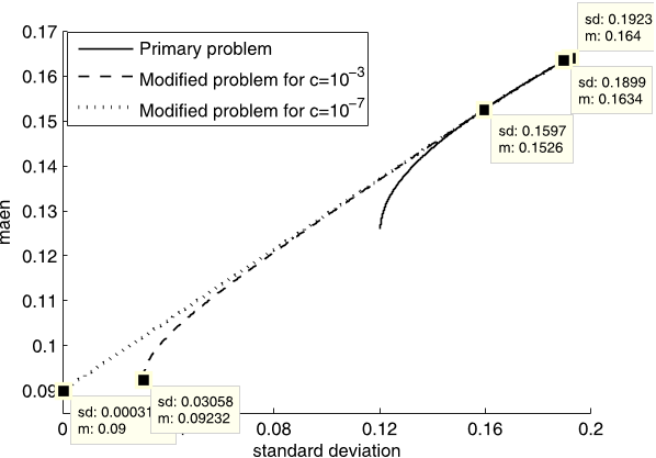
  • Theorem 3.2 implies that Problems 1 and 2 are equivalent for any ρ ∈ [ρ̂T , ρ̂max], in the sense that both problems have the same optimal portfolio, and consequently have the same efficient frontier (see Fig. 1).

4. The tangency portfolio as a corner portfolio

  • In this section the authors discuss some advantages of applying Problem 2 and describe their algorithm.
  • But, the authors can take more main steps to determine the exact location of ρT as described in the following.
  • Equations are considered as constraints that are always active.
  • An efficient portfolio is said to be a corner portfolio if in its vicinity on the efficient frontier, other efficient portfolios have different active sets, see [15].
  • The GMV portfolio, however, is included as a corner portfolio (last corner portfolio) irrespective of its active set.

4.1. Description of the algorithm

  • Now, the authors may use any relevant PQP algorithm, which produce corner portfolios, to determine the tangency portfolio as a corner portfolio.
  • For this, he used the Lagrangian multipliers generated by the CLA and applied the sign of θ(Λ) during the iterations of the method.
  • As mentioned before, for example, the algorithm of Niedermayer and Niedermayer [13] can compute the efficient frontier of the standard problem with 2000 assets in less than a second.
  • The authors use Optimizer to compute the corner portfolios.
  • Moreover, for values of c closed to zero, GMV portfolio acts like a totally riskless portfolio and that segment of the efficient frontier between the tangency portfolio and the GMV portfolio, tends to a straight line.

Did you find this useful? Give us your feedback
Content maybe subject to copyright    Report

RAIRO-Oper. Res. 47 (2013) 311–320 RAIRO Operations Research
DOI: 10.1051/ro/2013041 www.rairo-ro.org
PRODUCING THE TANGENCY PORTFOLIO
AS A CORNER PORTFOLIO
Reza Keykhaei
1
and Mohamad-Taghi Jahandideh
2
Abstract. One-fund theorem states that an efficient portfolio in a
Mean-Variance (M-V) portfolio selection problem for a set of some risky
assets and a riskless asset can be represented by a combination of a
unique risky fund (tangency portfolio) and the riskless asset. In this
paper, we introduce a method for which the tangency portfolio can
be produced as a corner portfolio. So, the tangency portfolio can be
computed easily and fast by any algorithm designed for tracing out the
M-V efficient frontier via computing the corner portfolios. Moreover,
we show that how this method can be used for tracing out the M-V
efficient frontier when problem contains a riskless asset in which the
borrowing is not allowed.
Keywords. M-V Optimization, Parametric Quadratic Programming,
Critical Line Algorithm, Capital Allocation Line, Tangency Portfolio.
Mathematics Subject Classification. 91G10, 90C20, 90C29.
1. Introduction
The aim of classic Mean-Variance (M-V) portfolio optimization, originated from
the seminal work of Markowitz [7], is to maximize the expected return of a portfolio
and minimize its variance as the measure of risk. Markowitz proposed his work for
a set of risky assets. M-V portfolio selection problems seek to compute efficient
portfolios. A portfolio is efficient if with respect to its location in the M-V space,
there is no obtainable portfolio with a lower variance without a lower expected
return or a greater expected return without a greater variance. The locus of all
Received July 4, 2012. Accepted July 11, 2013.
1
Department of Mathematics, Khansar Faculty of Computer and Mathematics, University
of Isfahan, Isfahan 81746-73441, Iran. r.keykhaei@math.iut.ac.ir
2
College of Mathematical Sciences, Isfahan University of Technology, 84156-83111, Isfahan,
Iran. jahandid@cc.iut.ac.ir
Article published by EDP Sciences
c
EDP Sciences, ROADEF, SMAI 2013

312 R. KEYKHAEI AND M.-T. JAHANDIDEH
efficient portfolios in the M-V plane is called the efficient frontier.Theideaof
riskless asset was first suggested by Tobin [16]. He included cash in his version of
portfolio selection problem and stated that any efficient portfolio is a combination
of a single risky fund and the riskless asset. This is the Tobin’s one-fund theorem.In
fact all combinations of a risky portfolio and a riskless asset can be represented by
a line, Capital Allocation Line (CAL), originating at the riskless asset and passing
through the risky portfolio, in the Mean-Standard Deviation (M-SD) plane. There
exists a CAL termed by optimal CAL, which dominates the other CALs. When
borrowing of riskless asset is allowed, the efficient frontier is the optimal CAL. The
optimal CAL has the highest possible slop and is tangent to the efficient frontier
of risky assets. We denote the risky portfolio corresponding to the tangent point
by the tangency portfolio. Indeed tangency portfolio is the efficient portfolio which
maximizes the famous Sharpe ratio [14]:
ρ r
f
σ
where, ρ and σ denotes the mean and the standard deviation of any efficient port-
folio, respectively, and r
f
denotes the return of the riskless asset. So, in order to
find the tangency portfolio it is enough to find efficient portfolios and recognize
the tangency portfolio which maximizes the Sharpe ratio (for example see chap-
ter seven of [3]). Markowitz [8] proposed his Critical Line Algorithm (CLA), as a
Parametric Quadratic Programming (PQP), for general portfolio selection mod-
els and developed it in his books [911], for computing the efficient portfolios.
Jacobs et al. [6] extended CLA to account for factor and scenario models with
realistic short positions. In addition to Markowits’s algorithm, there are other
PQP algorithms which proposed in the literature to trace out the M-V efficient
frontier, for example we can refer to Best [1], Stein et al. [15], Niedermayer and
Niedermayer [13] and Hirschberger et al. [5]. As we know, in the M-V plane, the
efficient frontier is consisting of connected parabolic segments. The portfolios cor-
responding to the end points of each segment are called corner portfolios. The
major aim of the above works is to introduce methods which calculate the cor-
ner portfolios and the efficient frontier while significantly reducing computational
time.
Todd programmed CLA algorithm in Visual Basic for Applications (VBA) and
the software is called Optimizer (see Markowitz and Todd [11]). Niedermayer
and Niedermayer [13] provide a Matlab quadratic optimization tool based on
Markowitz’s CLA. Their method computes the efficient frontier of the standard
problem with 2000 assets in less than a second.
ut¨unc¨u[17] presented a modification of the CLA which computes the tan-
gency portfolio as a by-product during the algorithm. In this paper, we present
an algorithm, based on T¨ut¨unc¨u’s results, for which the tangency portfolio can be
produced as a corner portfolio. So, the tangency portfolio, as a corner portfolio,
can be calculated in a short time using CLA (or other suitable methods). More-
over, we show that how this method can be used to trace out the efficient frontier

PRODUCING THE TANGENCY PORTFOLIO AS A CORNER PORTFOLIO 313
when portfolio contains a riskless asset and borrowing is not allowed for riskless
asset.
The paper proceeds is as follows. The M-V portfolio selection problem formu-
lation and the results of T¨ut¨unc¨u about the tangency portfolio are described in
Section 2. In Section 3 we describe the modified portfolio selection problem and
give the main results. in Section 4 we present our algorithm for finding the tan-
gency portfolio.
2. The tangency portfolio
Consider a portfolio consisting of n 2 risky assets with the random returns
r
1
,...,r
n
.Let
¯
R =(¯r
1
,...,¯r
n
)
and Σ be the mean vector and covariance matrix
of the asset returns, respectively. We denote each portfolio by the vector of asset
weights x := (x
1
,...,x
n
)
R
n
,whereeachx
i
is the weight allocated to the ith
asset. Here
¯
R
x and x
Σx are the expected return and the variance of the portfolio,
respectively. We assume that no asset can be represented by a linear combination
of other assets, which implies that Σ is positive definite. So, the variance is a
strictly convex function of portfolio variables. Also, we assume that not all of the
mean returns of the assets are equal. A portfolio x is feasible if it belongs to the
following set:
S = {x R
n
: Ax = b, Cx d} , (2.1)
where b R
m
, d R
p
, A is an m × n,andC is a p × n matrix over R.
The Markowitz portfolio selection problem, as a Quadratic Programming (QP)
problem, which corresponds to expected return ρ has the following form:
Problem 2.1.
min
x
1
2
x
Σx
s.t.
¯
R
x = ρ,
x S.
The model for S = {x R
n
: 1
x =1, x 0} is called the standard portfolio
selection model, where 1 is a vector of ones. Merton [12] considered the unbounded
portfolio weight model, i.e. S = {x R
n
: 1
x =1}, and give an analytical solution
for the problem.
By the Karush-Kuhn-Tucker (K-K-T) conditions, X
=(x
1
,...,x
n
)
is a (pri-
mal) solution or optimal portfolio of Problem 1, if and only if, there exist vectors
λ
ρ
R, λ
b
R
m
and λ
d
R
p
such that:
Σx
λ
ρ
¯
R A
λ
b
C
λ
d
=0,
¯
R
x
= ρ, Ax
= b
d
(Cx
d)=0,
Cx
d
d
0.
(2.2)

314 R. KEYKHAEI AND M.-T. JAHANDIDEH
We denote the primal-dual solution of Problem 1 by (x
ρ
b
d
)or(x
),
where Λ := (λ
ρ
b
d
). Since variance is strictly convex, x
is unique. Let us
denote the set of all primal-dual solutions of Problem 1 by Ω(ρ).
Let ρ
min
be the expected return of the Global Minimum-Variance (GMV) port-
folio which has the minimum variance between all feasible portfolios. We assume
that r
f
min
,wherer
f
is the return of the riskless asset. Also let ρ
max
be the
highest obtainable expected return of feasible portfolios and ρ
T
be the expected
return of the tangency portfolio. Actually, any efficient portfolio has expected re-
turn ρ [ρ
min
max
]. As in [17], we define function σ :[ρ
min
max
] R by
σ(ρ):=(x
Σx
)
1/2
;where(x
) Ω(ρ). In fact σ(ρ) represents the efficient
frontier. Note that σ(ρ) is convex but not necessarily smooth. In fact the efficient
frontier might have kinks, i.e., the points of nondifferentiability (see [2, 4, 18]).
Considering this, we refer to ∂σ(ρ), as the subdifferential of σ at ρ,and
L(R)=
λ
ρ
σ(ρ)
:(x
ρ
b
d
) Ω(ρ)
,
as stated in [17]. Now the following key theorem holds:
Theorem 2.2. L(R)=∂σ(ρ).Also,σ(ρ
T
)/(ρ
T
r
f
), the slope of the optimal
CAL, belongs to ∂σ(ρ
T
).
Proof. See Theorem 1 of [17] and the paragraph following the theorem.
For (x
) Ω(ρ) we define
θ(Λ):=r
f
λ
ρ
+ b
λ
b
+ d
λ
d
.
The next theorem states some results derived in [17].
Theorem 2.3. For any expected return ρ (ρ
T
max
], θ(Λ) < 0; and for any
expected return ρ [ρ
min
T
), θ(Λ) > 0.Alsoifθ(Λ)=0then, ρ = ρ
T
. Moreover
if θ(Λ) > 0(θ(Λ) < 0) for ρ = ρ
max
(ρ = ρ
min
) then ρ
max
= ρ
T
(ρ
min
= ρ
T
).
Proof. See Corollary 1 of [17] and the paragraph following the corollary.
The assertions of Theorem 2.3 are presented with respect to corresponding
Lagrangian multiplier of any optimal portfolio. We use the above theorem to get
similar results with respect to optimal asset weights.
3. The modified problem
In this section, we introduce the modified problem that corresponds to Problem
1, which contains an additional variable x
f
so-called free variable. In this case the
new portfolio is x
1
:= (x
1
,...,x
n
,x
f
)
R
n+1
. In the following we show x
1
by
(x,x
f
)wherex =(x
1
,...,x
n
)
.

PRODUCING THE TANGENCY PORTFOLIO AS A CORNER PORTFOLIO 315
Considering Problem 1, the modified portfolio selection problem for the ex-
pected return ρ is:
Problem 3.1.
min
x
1
1
2
x
1
Σ
1
x
1
s.t.
¯
R
1
x
1
= ρ,
x
1
S
1
,
where
S
1
=
x
1
R
n+1
: A
1
x
1
= b, C
1
x
1
d,x
f
0
, A
1
=
Ab
and
C
1
=
Cd
,
¯
R
1
=
¯
R
r
f
and
Σ
1
=
Σ 0
0 c
for the arbitrary constant c>0. (The value of c can be interpreted as the variance
of the return of the asset x
f
which its return is uncorrelated with the returns of
the other assets and has the expected value r
f
). The last two constraints in S
1
can be replaced by C
2
x
1
d
1
,where
C
2
=
Cd
01
and d
1
=
d
0
.
x
1
S
1
is called a feasible portfolio. Obviously x satisfies the conditions of Prob-
lem 1, if and only if, (x, 0) satisfies the conditions of Problem 2.
Let x
1
=(
ˆ
x,x
f
)and(
ˆ
x,x
f
,
ˆ
Λ):=(
ˆ
x,x
f
,
ˆ
λ
ρ
,
ˆ
λ
b
,
ˆ
λ
d
,
ˆ
λ
f
)denotethe(primal)
solution and a primal-dual solution of problem 2, respectively, then
Σ
ˆ
x
ˆ
λ
ρ
¯
R A
ˆ
λ
b
C
ˆ
λ
d
=0,
cx
f
¯r
f
ˆ
λ
ρ
b
ˆ
λ
b
d
ˆ
λ
d
=
ˆ
λ
f
,
¯
R
1
x
1
= ρ, A
1
x
1
= b,
ˆ
λ
d
(C
1
x
1
d)=0,
ˆ
λ
f
x
f
=0,
C
1
x
1
d,x
f
0,
ˆ
λ
d
0,
ˆ
λ
f
0.
(3.1)
We denote the set of all primal-dual solution of Problem 2 by
ˆ
Ω(ρ) and define
ˆ
θ(
ˆ
Λ):=r
f
ˆ
λ
ρ
+ b
ˆ
λ
b
+ d
1
ˆ
λ
I
,
where (
ˆ
x,x
f
,
ˆ
Λ)
ˆ
Ω(ρ)and
ˆ
λ
I
=(
ˆ
λ
d
,
ˆ
λ
f
)
.Notethat
ˆ
θ(
ˆ
Λ)=r
f
ˆ
λ
ρ
+ b
ˆ
λ
b
+ d
ˆ
λ
d
.
Let ˆρ
max
and ˆρ
min
be the maximum and the minimum obtainable expected
returns, respectively, and ˆρ
T
be the mean return of the tangency portfolio related
to Problem 2. Then the following theorem holds:
Theorem 3.2. If ρ ρ
T
, ˆρ
max
] then, x
f
=0.Also,x
f
> 0 for any ρ
ρ
min
, ˆρ
T
).

Citations
More filters
Posted Content
TL;DR: In this paper the standard portfolio case with short sales restrictions is analyzed and the sufficient condition is given here and a new procedure is used to derive the efficient frontier, i.e. the characteristics of the mean variance frontier.
Abstract: In this paper the standard portfolio case with short sales restrictions is analyzed.Dybvig pointed out that if there is a kink at a risky portfolio on the efficient frontier, then the securities in this portfolio have equal expected return and the converse of this statement is false.For the existence of kinks at the efficient frontier the sufficient condition is given here and a new procedure is used to derive the efficient frontier, i.e. the characteristics of the mean variance frontier.

4 citations

Posted Content
01 Jan 2017
TL;DR: In this paper, an empirical study which aims to test the Markowitz Modern portfolio theory (MPT) or the mean-variance analysis is presented. And the theoretical framework of Markowitz MPT tested by computed 134 months expected the return of thirtytwo stocks, thirty-one variances and 465 co-variances, in order to evaluate efficient portfolio frontier.
Abstract: Basically this is an empirical study which aims to test the Markowitz Modern portfolio theory (MPT) or the mean-variance analysis. Fund managers and general investors seek a portfolio that yields maximum return with minimum risk. The problem of investors is dual in nature, as Markowitz showed, i.e., the indifferent choice of risk and return. Though, diversification reduces non-systematic risk but due to limited resources one cannot afford to invest in all stocks, therefore it is pertinent to know that what should be the minimum level of stocks in a portfolio that produces maximum return and minimum risk. The theoretical framework of Markowitz MPT tested by computed 134 months expected the return of thirtytwo stocks, thirty-one variances and 465 co-variances, in order to evaluate efficient portfolio frontier.

1 citations


Cites background from "Producing the tangency portfolio as..."

  • ...As Keykhaei and Jahandideh (2013) pointed out that, in fact all combinations of a risky portfolio and a riskless asset can be represented by a line - Capital Allocation Line (CAL), originating at the riskless asset and passing through the risky portfolio, in the Mean-Standard Deviation (M-SD) plane....

    [...]

  • ...As pointed out by Keykhaei and Jahandideh (2013) ‘in order to find the tangency portfolio, it is enough to find the efficient portfolios and recognize the tangency portfolios which maximizes the Sharpe ratio’....

    [...]

References
More filters
Journal ArticleDOI
TL;DR: This note shows how a simple modification of Markowitz' method of critical lines can be used to determine the optimal risky portfolio in a faster, more reliable, and more memory-efficient way than the standard approaches.
Abstract: Given a number of risky assets and a riskless asset, the set of efficient portfolios in the mean-variance optimization sense are combinations of the riskless asset and a unique optimal risky portfolio. This note shows how a simple modification of Markowitz' method of critical lines can be used to determine the optimal risky portfolio in a faster, more reliable, and more memory-efficient way than the standard approaches.

6 citations


"Producing the tangency portfolio as..." refers background or methods or result in this paper

  • ...Tütüncü [17] presented a modification of the CLA which computes the tangency portfolio as a by-product during the algorithm....

    [...]

  • ...As in [17], we define function σ : [ρmin, ρmax] → R by σ(ρ) := (x∗′Σx∗)1/2; where (x∗, Λ) ∈ Ω(ρ)....

    [...]

  • ...See Theorem 1 of [17] and the paragraph following the theorem....

    [...]

  • ...The next theorem states some results derived in [17]....

    [...]

  • ...Tütüncü [17] presented an algorithm using CLA to calculate the tangency portfolio....

    [...]

Posted Content
TL;DR: In this paper the standard portfolio case with short sales restrictions is analyzed and the sufficient condition is given here and a new procedure is used to derive the efficient frontier, i.e. the characteristics of the mean variance frontier.
Abstract: In this paper the standard portfolio case with short sales restrictions is analyzed.Dybvig pointed out that if there is a kink at a risky portfolio on the efficient frontier, then the securities in this portfolio have equal expected return and the converse of this statement is false.For the existence of kinks at the efficient frontier the sufficient condition is given here and a new procedure is used to derive the efficient frontier, i.e. the characteristics of the mean variance frontier.

4 citations


Additional excerpts

  • ..., the points of nondifferentiability (see [2, 4, 18])....

    [...]

Journal ArticleDOI
TL;DR: In this article, the standard portfolio case with short sales restrictions is analyzed and a new procedure is used to derive the efficient frontier, i.e. the characteristics of the mean variance frontier.

4 citations

Frequently Asked Questions (12)
Q1. What have the authors contributed in "Producing the tangency portfolio as a corner portfolio" ?

In this paper, the authors introduce a method for which the tangency portfolio can be produced as a corner portfolio. Moreover, the authors show that how this method can be used for tracing out the M-V efficient frontier when problem contains a riskless asset in which the borrowing is not allowed. 

for values of c closed to zero, GMV portfolio acts like a totally riskless portfolio and that segment of the efficient frontier between the tangency portfolio and the GMV portfolio, tends to a straight line. 

The major aim of the above works is to introduce methods which calculate the corner portfolios and the efficient frontier while significantly reducing computational time. 

Also when portfolio contains a riskless asset with rf = 0.09 and borrowing is not allowed, the efficient frontier contains x11,x 2 1,x 3 1 and x 0 1 as the corner portfolios, where x01 corresponds to the totally riskless investment, i.e., (0,0.09), on the mean axis. 

Note that, since x∗f = 0 for any ρ ≥ ρT and x∗f > 0 for any ρ < ρT , the tangency portfolio is a corner portfolio in the modified problem. 

Since problems 1 and 2 have the same efficient frontiers on [ρ̂T , ρmax] and the efficient frontier of Problem 2 strictly dominates the efficient frontier of Problem 1 on [ρmin, ρ̂T ), the optimal CAL corresponding to Problem 2 which is tangent to the efficient frontier of the problem, is also tangent to the efficient frontier of Problem 1. 

their model works directly with the optimal asset weights, instead of the Lagrangian multipliers, which is more clear to express, and also can employ other suitable PQP algorithms. 

the efficient frontier of Problem 2 strictly dominates the efficient frontier of Problem 1 when ρ < ρ̂T .Corollary 3.3. ρmax = ρ̂max, where both of the problems 1 and 2 have the same optimal portfolio. 

By the Karush-Kuhn-Tucker (K-K-T) conditions, X∗ = (x∗1, . . . , x∗n)′ is a (primal) solution or optimal portfolio of Problem 1, if and only if, there exist vectors λρ ∈ R, λb ∈ Rm and λd ∈ Rp such that:Σx∗ − λρR̄ − A′λb − C′λd = 0, R̄′x∗ = ρ, 

As mentioned before, for example, the algorithm of Niedermayer and Niedermayer [13] can compute the efficient frontier of the standard problem with 2000 assets in less than a second. 

Observe thatλ̂ρ̂T (ρ̂T − rf ) = x̂′Σx̂′ + cx∗f 2 = ρ̂T λ̂ρ̂T + b′λ̂b + d′λ̂d,where the last equation is obtained by adding the two first equations of (3.1) multiplied by x̂′ and x∗f , respectively. 

the authors can locate the expected return of the tangency portfolio associated with Problem 1, which is also the tangency portfolio associated with Problem 2 (Cor. 3.4), by looking at the value of free variable in the solution of Problem 2.