scispace - formally typeset
Search or ask a question
Journal ArticleDOI

Sampling-50 years after Shannon

01 Apr 2000-Vol. 88, Iss: 4, pp 569-587
TL;DR: The standard sampling paradigm is extended for a presentation of functions in the more general class of "shift-in-variant" function spaces, including splines and wavelets, and variations of sampling that can be understood from the same unifying perspective are reviewed.
Abstract: This paper presents an account of the current state of sampling, 50 years after Shannon's formulation of the sampling theorem. The emphasis is on regular sampling, where the grid is uniform. This topic has benefitted from a strong research revival during the past few years, thanks in part to the mathematical connections that were made with wavelet theory. To introduce the reader to the modern, Hilbert-space formulation, we reinterpret Shannon's sampling procedure as an orthogonal projection onto the subspace of band-limited functions. We then extend the standard sampling paradigm for a presentation of functions in the more general class of "shift-in-variant" function spaces, including splines and wavelets. Practically, this allows for simpler-and possibly more realistic-interpolation models, which can be used in conjunction with a much wider class of (anti-aliasing) prefilters that are not necessarily ideal low-pass. We summarize and discuss the results available for the determination of the approximation error and of the sampling rate when the input of the system is essentially arbitrary; e.g., nonbandlimited. We also review variations of sampling that can be understood from the same unifying perspective. These include wavelets, multiwavelets, Papoulis generalized sampling, finite elements, and frames. Irregular sampling and radial basis functions are briefly mentioned.

Summary (4 min read)

Introduction

  • The emphasis is on regular sampling, where the grid is uniform.
  • Recently, there has been strong revival of the subject, which was motivated by the intense activity taking place around wavelets (see [7], [35], [80], and [85]).

II. SHANNON’S SAMPLING THEOREM REVISITED

  • Shannon’s sampling theory is applicable whenever the input function is bandlimited.
  • The optimal choice is the ideal filter , which suppresses aliasing completely without introducing any distortion in the bandpass region.
  • In 1941, the English mathematician Hardy, who was referring to the basis functions in Whittaker’s cardinal series (1), wrote: “It is odd that, although these functions occur repeatedly in analysis, especially in the theory of interpolation, it does not seem to have been remarked explicitly that they form an orthogonal system” [55].
  • This orthonormality property greatly simplifies the implementation of the approximation process by which a function is projected onto .
  • The conclusion of this section is that the traditional sampling paradigm with ideal prefiltering yields an approximation , which is the orthogonal projection of the input function onto (the space of band-limited functions).

B. Minimum Error Sampling

  • Having defined their signal space, the next natural question is how to obtain the ’s in (9) such that the signal model is a faithful approximation of some input function .
  • The optimal solution in the least squares sense is the orthogonal projection, which can be specified as (18) where the ’s are the dual basis functions of .
  • This is very similar to (6), except that theanalysisandsynthesisfunctions ( and , respectively) are not identical—in general, the approximation problem is not decoupled.
  • It also inherits the translation-invariant structure of the basis functions: .
  • Similar to what has been said for the band-limited case [see (4)], the algorithm described by (18) has a straightforward signal-processing interpretation (see Fig. 2).

C. Consistent Sampling

  • The authors have just seen how to design an optimal sampling system.
  • Provided there exists such that , then there is a unique signal approximationin that is consistent with in the sense that (23).
  • The projection property implies that the method can reconstruct perfectly any signal that is included in the reconstruction space; i.e., , .
  • To model the sampling process, the authors take the analysis function to be (Dirac delta).
  • The interpolating signal that results from this process is This solution can also be presented in a form closer to the traditional one [see (1)] (30) where is the interpolation function given by (31).

E. Equivalent Basis Functions

  • So far, the authors have encountered three types of basis functions: the generic ones , the duals ( ), and the interpolating ones ( ).
  • Interestingly, it has been shown that the interpolator and the orthonormal function associated with many families of function spaces (splines, Dubuc–Deslaurier [42], etc.) both converge to Shannon’s sinc interpolator as the order (to be defined in Section IV-B) tends to infinity [9], [10], [130].
  • If one is only concerned with the signal values at the integers, then the so-called cardinal representation is the most adequate; here, the knowledge of the underlying basis function is only necessary when one wishes to discretize some continuous signal-processing operator (an example being the derivative) [122].
  • Another interesting aspect is the time-frequency localization of the basis functions.
  • Furthermore, by using this type of basis function in a wavelet decomposition (see Section V-A), it is possible to trade one type of resolution for the other [31], [129].

F. Sampling and Reproducing Kernel Hilbert Spaces

  • The authors now establish the connection between what has been presented so far and Yao and Nashed’s general formulation of sampling using reproducing kernel Hilbert spaces (RKHS’s) [87], [148].
  • The reproducing kernel for a given Hilbert spaceis unique; is is also symmetric .
  • The authors now show how these can be constructed with the help of Theorem 2.
  • The oblique projection operator (24) may therefore be written in a form similar to (18) Formally, this is equivalent to where the authors have now identified the projection kernel (37).
  • Note that it is the inclusion constraint (33) that specifies the reprodcuing kernel in a unique fashion.

G. Extension to Higher Dimensions

  • All results that have been presented carry over directly for the representation of multidimensional signals (or images) , provided that the sampling is performed on the cartesian grid .
  • This generalization holds because their basic mathematical tool, Poisson’s summation formula , remains valid in dimensions.
  • In practice, one often uses separable generating functions of the form.
  • This greatly simplifies the implementation because all filtering operations are separable.
  • The dual functions remain separable as well.

IV. CONTROLLING THE APPROXIMATION ERROR

  • The projection interpretation of the sampling process that has just been presented has one big advantage: it does not require the band-limited hypothesis and is applicable for any function .
  • For more general spline-like spaces , the situation is more complicated.
  • This has led researchers in signal processing, who wanted a simple way to determine the critical sampling step, to develop an accurate error estimation technique which is entirely Fourier-based [20], [21].
  • This recent method is easy to apply in practice and yet powerful enough to recover most classical error bounds; it will be described next.
  • The key parameter for controlling the approximation error is the sampling step .

A. Calculating the Error in the Frequency Domain

  • Let denote a linear approximation operator with sampling step .
  • This corresponds to the general sampling system described in Fig. 2 and includes all the algorithms described so far.
  • In other words,Q commutes with the shift operator by integer multiples ofT .
  • For the standard Shannon paradigm, which uses ideal analysis and reconstruction filters, the authors find that ; this confirms the fact that the approximation error is entirely due to the out-of-band portion of the signal.
  • The -approximation error of the operator defined by can be written as (44) where is a correction term negligible under most circumstances.

C. Comparison of Approximation Algorithms

  • The leading constant in (45) for linear spline interpolation is ; this is more than a factor of two above the projection algorithms b) and c), which both achieve the smallest possible constant .
  • More generally, it has been shown that the performances ofth order orthogonal and oblique projectors are asymptotically equivalent, provided that the analysis and synthesis functions are biorthogonal and that satisfies the partition of unity [123].
  • Under those hypotheses, the leading constant in (45) is given by (46) where denotes the th derivative of the Fourier transform of .
  • A simpler and more direct formula in terms of the refinement filter is available for wavelets [20].

D. Comparison of Approximation Spaces

  • The other interesting issue that the authors may address using the above approximation results is the comparison of approxi- mation subspaces.
  • As increases, the spline approximation converges to Shannon’s band-limited solution [130].
  • The last three generating functions are of order and are members of the so-called Moms (maximum order minimum support) family; the cubic spline is the smoothest member while the O-Moms is the one with the smallest asymptotic constant (46), which explains its better performance.
  • The state-of-the art interpolation method in image processing [91], [94], but the situation is likely to change.
  • For a more classical perspective on sampling, the authors refer to Jerri’s excellent tutorial article, which gives a very comprehensive view of the subject up to the mid 1970’s [62].

B. Generalized (or Multichannel) Sampling

  • In 1977, Papoulis introduced a powerful extension of Shannon’s sampling theory, showing that a band-limited signal could be reconstructed exactly from the samples of the response of linear shift-invariant systems sampled at 1 the reconstruction rate [90].
  • If the measurements are performed in a structured manner, then the reconstruction process is simplified: for example, in the Papoulis framework, it is achieved by multivariate filtering [23], [83].
  • Typical instances of generalized sampling are interlaced and derivative sampling [75], [149], both of which are special cases of Papoulis’ formulation.
  • More recently, Papoulis’ theory has been generalized in several directions.
  • While still remaining with band-limited functions, it was extended for multidimensional, as well as multicomponent signals [25], [101].

C. Finite Elements and Multiwavelets

  • To obtain a signal representation that has the same sampling density as before, the multifunctions are translated by integer multiples of (48).
  • In the more recent multiwavelet constructions, the multiscaling functions satisfy a vector two-scale relation—similar to (17)—that involves a matrix refinement filter instead of a scalar one [4], [45], [51], [56], [116].
  • The situation is very much the same as in the scalar case, when the generating function is noninterpolating (see Section III-D).
  • Given the equidistant samples (or measurements) of a signal , the expansion coefficients are usually obtained through an appropriate digital prefiltering procedure (analysis filterbank) [54], [140], [146].
  • Because of the importance of the finite elements in engineering, the quality of this type of approximation has been studied thoroughly by approximation theorists [64], [73], [111].

D. Frames

  • The notion of frame, which generalizes that of a basis, was introduced by Duffin and Schaffer [47]; it plays a crucial role in nonuniform sampling [12].
  • The main difference with the Riesz basis condition (10) is that the frame definition allows for redundancy: there may be more template functions than are strictly necessary.
  • Practically, the signal reconstruction is obtained from the solution of an overdetermined system of linear equations [92]; see also [34], for an iterative algorithm whenis close to .
  • Irregular Sampling Irregular or nonuniform sampling constitutes another whole area of research that the authors mention here only briefly to make the connection with what has been presented.
  • 2) Nonuniform Splines and Radial Basis Functions:.

VI. CONCLUSION

  • Fifty years later, Shannon’s sampling theory is still alive and well.
  • 4, APRIL 2000 communications including the Web, sound, television, photography, multimedia, medical imaging, etc.
  • Many of the results reviewed in this paper have a potential for being useful in practice because they allow for a realistic modeling of the acquisition process and offer much more flexibility than the traditional band-limited framework.
  • Last, the authors believe that the general unifying view of sampling that has emerged during the past decade is beneficial because it offers a common framework for understanding—and hopefully improving—many techniques that have been traditionally studied by separate communities.
  • Areas that may benefit from these developments are analog-to-digital conversion, signal and image processing, interpolation, computer graphics, imaging, finite elements, wavelets, and approximation theory.

Did you find this useful? Give us your feedback

Content maybe subject to copyright    Report

Sampling—50 Years After Shannon
MICHAEL UNSER, FELLOW, IEEE
This paper presents an account of the current state of sampling,
50 years after Shannon’s formulation of the sampling theorem. The
emphasis is on regular sampling, where the grid is uniform. This
topic has benefited from a strong research revival during the past
few years, thanks in part to the mathematical connections that were
made with wavelet theory. To introduce the reader to the modern,
Hilbert-space formulation, we reinterpret Shannon’s sampling pro-
cedure as an orthogonal projection onto the subspace of band-lim-
ited functions. We then extend the standard sampling paradigm for
a representation of functions in the more general class of “shift-in-
variant” functions spaces, including splines and wavelets. Practi-
cally, this allows for simpler—and possibly more realistic—inter-
polation models, which can be used in conjunction with a much
wider class of (anti-aliasing) prefilters that are not necessarily ideal
low-pass. We summarize and discuss the results available for the
determination of the approximation error and of the sampling rate
when the input of the system is essentially arbitrary; e.g., nonban-
dlimited. We also review variations of sampling that can be under-
stood from the same unifying perspective. These include wavelets,
multiwavelets, Papoulis generalized sampling, finite elements, and
frames. Irregular sampling and radial basis functions are briefly
mentioned.
Keywords—Band-limited functions, Hilbert spaces, interpola-
tion, least squares approximation, projection operators, sampling,
sampling theorem, Shannon, splines, wavelets.
I. INTRODUCTION
In 1949, Shannon published the paper “Communication in
the Presence of Noise,” which set the foundation of informa-
tion theory [105], [106]. This paper is a masterpiece; both in
terms of achievement and conciseness. It is undoubtedly one
of the theoretical works that has had the greatest impact on
modern electrical engineering [145]. In order to formulate his
rate/distortion theory, Shannon needed a general mechanism
for converting an analog signal into a sequence of numbers.
This led him to state the classical sampling theorem at the
very beginning of his paper in the following terms.
Theorem 1 [Shannon]: If a function
contains no fre-
quencies higher than
(in radians per second), it is com-
pletely determined by giving its ordinates at a series of points
spaced
seconds apart.
Manuscript received September 17, 1999; revised January 4, 2000.
The author is with the Biomedical Imaging Group, Swiss Federal Institute
of Technology Lausanne CH-1015 Lausanne EPFL, Switzerland (e-mail:
Michael.Unser@epfl.ch).
Publisher Item Identifier S 0018-9219(00)02874-7.
While Shannon must get full credit for formalizing this
result and for realizing its potential for communication
theory and for signal processing, he did not claim it as his
own. In fact, just below the theorem, he wrote: “this is a
fact which is common knowledge in the communication
art.” He was also well aware of equivalent forms of the
theorem that had appeared in the mathematical literature;
in particular, the work of Whittaker [144]. In the Russian
literature, this theorem was introduced to communication
theory by Kotel’nikov [67], [68].
The reconstruction formula that complements the sam-
pling theorem is
(1)
in which the equidistant samples of
may be interpreted
as coefficients of some basis functions obtained by appro-
priate shifting and rescaling of the sinc-function: sinc
. Formula (1) is exact if is bandlimited to
; this upper limit is the Nyquist frequency, a
term that was coined by Shannon in recognition of Nyquist’s
important contributions in communication theory [88]. In the
mathematical literature, (1) is known as the cardinal series
expansion; it is often attributed to Whittaker in 1915 [26],
[143] but has also been traced back much further [14], [58].
Shannon’s sampling theorem and its corresponding recon-
struction formula are best understood in the frequency do-
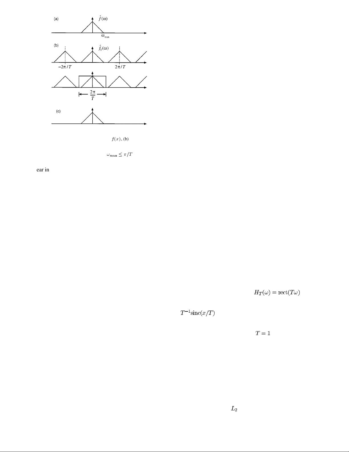
main, as illustrated in Fig. 1. A short reminder of the key
sampling formulas is provided in Appendix A to make the
presentation self-contained.
Nowadays the sampling theorem plays a crucial role in
signal processing and communications: it tells us how to
convert an analog signal into a sequence of numbers, which
can then be processed digitally—or coded—on a computer.
While Shannon’s result is very elegant and has proven to
be extremely fruitful, there are several problems associated
with it. First, it is an idealization: real world signals or
images are never exactly bandlimited [108]. Second, there is
no such device as an ideal (anti-aliasing or reconstruction)
low-pass filter. Third, Shannon’s reconstruction formula is
rarely used in practice (especially with images) because of
the slow decay of the sinc function [91]. Instead, practi-
tioners typically rely on much simpler techniques such as
0018–9219/00$10.00 © 2000 IEEE
PROCEEDINGS OF THE IEEE, VOL. 88, NO. 4, APRIL 2000 569

Fig. 1. Frequency interpretation of the sampling theorem: (a)
Fourier transform of the analog input signal
f
(
x
)
, (b) the sampling
process results in a periodization of the Fourier transform, and (c)
the analog signal is reconstructed by ideal low-pass filtering; a
perfect recovery is possible provided that
!
=T
.
linear interpolation. Despite these apparent mismatches with
the physical world, we will show that a reconciliation is
possible and that Shannon’s sampling theory, in its modern
and extended versions, can perfectly handle such “nonideal”
situations.
Ten to 15 years ago, the subject of sampling had reached
what seemed to be a very mature state [26], [62]. The re-
search in this area had become very mathematically oriented,
with less and less immediate relevance to signal processing
and communications. Recently, there has been strong revival
of the subject, which was motivated by the intense activity
taking place around wavelets (see [7], [35], [80], and [85]).
It soon became clear that the mathematics of wavelets were
also applicable to sampling, but with more freedom because
no multiresolution is required. This led researchers to reex-
amine some of the foundations of Shannon’s theory and de-
velop more general formulations, many of which turn out to
be quite practical from the point of view of implementation.
Our goal in this paper is to give an up-to-date account of
the recent advances that have occurred in regular sampling.
Here, the term “regular” refers to the fact that the samples
are taken on a uniform grid—the situation most commonly
encountered in practice. While the paper is primarily con-
ceived as a tutorial, it contains a fair amount of review mate-
rial—mostly recent work: This should make it a useful com-
plement to the excellent survey article of Jerri, which gives
a comprehensive overview of sampling up to the mid-1970’s
[62].
The outline of this paper is as follows. In Section II, we
will argue that the requirement of a perfect reconstruction
is an unnecessarily strong constraint. We will reinterpret the
standard sampling system, which includes an anti-aliasing
prefilter, as an orthogonal projection operator that computes
the minimum error band-limited approximation of a not-nec-
essarily band-limited input signal. This is a crucial obser-
vation that changes our perspective: instead of insisting that
the reconstruction be exact, we want it to be as close as pos-
sible to the original; the global system, however, remains un-
changed, except that the input can now be arbitrary. (We can
obviously not force it to be bandlimited.)
In Section III, we will show that the concept extends nicely
to the whole class of spline-like (or wavelet-like) spaces gen-
erated from the integer shifts of a generating function. We
will describe several approximation algorithms, all based on
the standard three-step paradigm: prefiltering, sampling, and
postfiltering—the only difference being that the filters are
not necessarily ideal. Mathematically, these algorithms can
all be described as projectors. A direct consequence is that
they reconstruct all signals included within the reconstruc-
tion space perfectly—this is the more abstract formulation
of Shannon’s theorem.
In Section IV, we will investigate the issue of approxima-
tion error, which becomes relevant once we have given up
the goal of a perfect reconstruction. We will present recent
results in approximation theory, making them accessible to
an engineering audience. This will give us the tools to select
the appropriate sampling rate and to understand the effect of
different approximation or sampling procedures.
Last, in Section V, we will review additional extensions
and variations of sampling such as (multi)wavelets, finite el-
ements, derivative and interlaced sampling, and frames. Ir-
regular sampling will also be mentioned, but only briefly, be-
cause it is not the main focus of this paper. Our list of sam-
pling topics is not exhaustive—for instance, we have com-
pletely left out the sampling of discrete sequences and of
stochastic processes—but we believe that the present paper
covers a good portion of the current state of research on
regular sampling. We apologize in advance to those authors
whose work was left out of the discussion.
II. S
HANNON’S SAMPLING THEOREM REVISITED
Shannon’s sampling theory is applicable whenever the
input function is bandlimited. When this is not the case, the
standard signal-processing practice is to apply a low-pass
filter prior to sampling in order to suppress aliasing. The
optimal choice is the ideal filter
, which
suppresses aliasing completely without introducing any
distortion in the bandpass region. Its impulse response is
. The corresponding block diagram is shown
in Fig. 2. In this section, we provide a geometrical Hilbert
space interpretation of the standard sampling paradigm. For
notational simplicity, we will set
and rescale the time
dimension accordingly.
In 1941, the English mathematician Hardy, who was re-
ferring to the basis functions in Whittaker’s cardinal series
(1), wrote: “It is odd that, although these functions occur re-
peatedly in analysis, especially in the theory of interpolation,
it does not seem to have been remarked explicitly that they
form an orthogonal system” [55]. Orthonormality is a fun-
damental property of the sinc-function that has been revived
recently.
To understand the modern point of view, we have to con-
sider the Hilbert space
, which consists of all functions that
570 PROCEEDINGS OF THE IEEE, VOL. 88, NO. 4, APRIL 2000

Fig. 2. Schematic representation of the standard three-step
sampling paradigm with
T
=1
: 1) the analog input signal is
prefiltered with
h
(
x
)
(anti-aliasing step), 2) the sampling process
yields the sampled representation
c
(
x
)=
c
(
k
)
(
x
0
k
)
,
and 3) the reconstructed output
~
f
(
x
)=
c
(
k
)
'
(
x
0
k
)
is obtained by analog filtering of
c
with
'
. In the traditional
approach, the pre- and postfilters are both ideal low-pass:
h
(
x
)=
'
(
x
)=sinc(
x
)
. In the more modern schemes, the filters
can be selected more freely under the constraint that they remain
biorthogonal:
h
'
(
x
0
k
)
;
~
'
(
x
0
l
)
i
=
.
are squareintegrable in Lebesgue’s sense. The corresponding
-norm is
(2)
It is induced by the conventional
-inner product
(3)
We now assume that the input function that we want to
sample is in
, a space that is considerably larger than the
usual subspace of band-limited functions, which we will
refer to as
. This means that we will need to make an
approximation if we want to represent a non-band-limited
signal in the band-limited space
. To make an analogy,
is to what (the real numbers) is to (the integers).
The countable nature of
is apparent if we rewrite the
normalized form of (1) with
as
with (4)
where the
’s are some coefficients, and where the ’s
are the basis functions to which Hardy was referring. It is not
difficult to show that they are orthonormal
(5)
where the autocorrelation function is evaluated as follows:
This orthonormality property greatly simplifies the imple-
mentation of the approximation process by which a function
is projected onto . Specifically, the orthogonal pro-
jection operator
can be written as
(6)
where the inner product
represents the signal
contribution along the direction specified by
—the ap-
proximation problem is decoupled component-wise because
of the orthogonality of the basis functions. The projection
theorem (see [69]) ensures that this projection operation is
well defined and that it yields the minimum-error approxi-
mation of
into .
(7)
By a lucky coincidence, this inner product computation is
equivalent to first filtering the input function
with the ideal
low-pass filter and sampling thereafter. More generally, we
observe that any combination of prefiltering and sampling
can be rewritten in terms of inner products
with (8)
That is, the underlying analysis functions correspond to the
integer shifts of
, the time-reversed impulse
response of the prefilter
(which can be arbitrary). In the
present case,
and is the
ideal low-pass filtered version of
.
The conclusion of this section is that the traditional sam-
pling paradigm with ideal prefiltering yields an approxima-
tion
, which is the orthogonal projection of the
input function onto
(the space of band-limited functions).
In other words,
is the approximation of in with min-
imum error. In light of this geometrical interpretation, it is
obvious that
(since is a projection
operator), which is a more concise statement of Shannon’s
theorem.
III. S
AMPLING IN SHIFT-INVARIANT (OR SPLINE-LIKE)
S
PACES
Having reinterpreted the sampling theorem from the more
abstract perspective of Hilbert spaces and of projection op-
erators, we can take the next logical step and generalize the
approach to other classes of functions.
A. Extending Shannon’s Model
While it would be possible to consider arbitrary basis func-
tions, we want a sampling scheme that is practical and retains
the basic, shift-invariant flavor of the classical theory. This is
achieved by simply replacing
by a more general tem-
plate: the generating function
. Accordingly, we specify
our basic approximation space
as
(9)
This means that any function
, which is con-
tinuously defined, is characterized by a sequence of coeffi-
cients
; this is the discrete signal representation that will
be used to do signal processing calculations or to perform
coding. Note that the
’s are not necessarily the samples
UNSER: SAMPLING—50 YEARS AFTER SHANNON 571

of the signal, and that can be something quite different
from
. Indeed, one of our motivations is to discover
functions that are simpler to handle numerically and have a
much faster decay.
For such a continuous/discrete model to make sense, we
need to put a few mathematical safeguards. First, the se-
quence of coefficients must be square-summable:
.
Second, the representation should be stable
1
and unambigu-
ously defined. In other words, the family of functions
should form a Riesz basis of , which
is the next best thing after an orthogonal one [35]. The def-
inition of a Riesz basis is that there must exist two strictly
positive constants
and such that
(10)
where
is the squared -norm (or en-
ergy) of
. A direct consequence of the lower inequality
is that
implies . Thus, the basis
functions are linearly independent, which also means that
every signal
is uniquely specified by its co-
efficients
. The upper bound in (10) implies that the
-norm of the signal is finite, so that is a valid sub-
space of
. Note that the basis is orthonormal if and only if
, in which case we have a perfect norm equiva-
lence between the continuous and the discrete domains (Par-
seval’s relation). Because of the translation-invariant struc-
ture of the construction, the Riesz basis requirement has an
equivalent expression in the Fourier domain [9]
(11)
where
is the Fourier transform of
. Note that the central term in (11) is the Fourier trans-
form of the sampled autocorrelation function
(12)
It can therefore also be written
[see (A.7) in Appendix A].
The final requirement is that the model should have the
capability of approximating any input function as closely as
desired by selecting a sampling step that is sufficiently small
(similar to the Nyquist criterion
). As shown
in Appendix B, this is equivalent to the partition of unity
condition
(13)
In practice, it is this last condition that puts the strongest
constraint of the selection on an admissible generating func-
tion
.
Let usnow lookat some examples. The firstone, which has
already been discussed in great length, is the classical choice
1
By stable, we mean that a small variation of the coefficients must result
in a small variation of the function. Here, the upper bound of the Riesz con-
dition (10) ensures
L
-stability.
. It is easy to verify that the corresponding
Riesz bounds in (11) are
, which is consistent
with the orthonormality property (5). We now show that the
sinc function satisfies the partition of unity: using Poisson’s
summation formula (cf. Appendix A), we derive an equiva-
lent formulation of (13) in the Fourier domain
2
(14)
a relation that is obviously satisfied by
, the
Fourier transform of
.
The sinc functionis well localized in the frequencydomain
but has very poor time decay. At the other extreme, we can
look for the simplest and shortest function that satisfies (13).
It is the box function (or B-spline of degree 0)
.
(15)
The corresponding basis functions are clearly orthogonal for
they do not overlap.
By convolving this function with itself repeatedly, we con-
struct the B-splines of degree
, which are defined recur-
sively as
(16)
These functions are known to generate the polynomial
splines with equally spaced knots [98], [99]. Specifically,
if
, then the signals defined by (9) are
polynomials of degree
within each interval (
odd), respectively, (1/2) (1/2) when is even,
with pieces that are patched together such as to guarantee
the continuity of the function and its derivatives up to order
(i.e., ). The B-spline basis functions up
to degree 4 are shown in Fig. 3. They are symmetric and
well localized, but not orthogonal—except for
. Yet,
they all satisfy the Riesz basis condition and the partition
of unity. This last property is easily verified in the Fourier
domain using (14). The B-splines are frequently used in
practice (especially for image processing) because of their
short support and excellent approximation properties [126].
The B-spline of degree 1 is the tent function, and the
corresponding signal model is piecewise linear. This rep-
resentation is quite relevant because linear interpolation is
one of the most commonly used algorithm for interpolating
signal values.
As additional examples of admissible generating func-
tions, we may consider any scaling function (to be defined
below) that appears in the theory of the wavelet transform
[35], [79], [115], [139]. It is important to note, however,
that scaling functions, which are often also denoted by
, satisfy an additional two-scale relation, which is
not required here but not detrimental either. Specifically,
a scaling function is valid (in the sense defined by Mallat
2
The equality on the right hand side of (14) holds in the distributional
sense provided that
'
(
x
)
2
L
, or by extension, when
'
(
x
)+
'
(
x
+1)
2
L
, which happens to be the case for
'
(
x
)=sinc(
x
)
572 PROCEEDINGS OF THE IEEE, VOL. 88, NO. 4, APRIL 2000

Fig. 3. The centered B-splines for
n
=0
to
4
. The B-splines of
degree
n
are supported in the interval
[
0
((
n
+1)
=
2)
;
((
n
+1)
=
2)]
;
as
n
increases, they flatten out andget more and more Gaussian-like.
[81]) if and only if 1) it is an admissible generating function
(Riesz basis condition
partition of unity) and 2) it satisfies
the two-scale relation
(17)
where
is the so-called refinement filter. In other words,
the dilated version of
must live in the space , a prop-
erty that is much more constraining than the conditions im-
posed here.
B. Minimum Error Sampling
Having defined our signal space, the next natural question
is how to obtain the
’s in (9) such that the signal model
is a faithful approximation of some input function
. The optimal solution in the least squares sense is the
orthogonal projection, which can be specified as
(18)
where the
’s are the dual basis functions of .
This is very similar to (6), except that the analysis and syn-
thesis functions (
and , respectively) are not identical—in
general, the approximation problem is not decoupled. The
dual basis
with is unique and is deter-
mined by the biorthogonality condition
(19)
It also inherits the translation-invariant structure of the basis
functions:
.
Since
, it is a linear conbination of the ’s.
Thus, we may represent it as
where is a suitable sequence to be determined next. Let
us therefore evaluate the inner product
where is the autocorrelation sequence in (12). By
imposing the biorthogonality constraint
,
and by solving this equation in the Fourier domain [i.e.,
], we find
that
(20)
Note that the Riesz basis condition (11) guarantees that this
solution is always well defined [i.e., the numerator on the
right-hand side of (20) is bounded and nonvanishing].
Similar to what hasbeensaid for the band-limited case [see
(4)], the algorithm described by (18) has a straightforward
signal-processing interpretation (see Fig. 2). The procedure
is exactly the same as the one dictated by Shannon’s theory
(with anti-aliasing filter), except that the filters are not nec-
essarily ideal anymore. Note that the optimal analysis filter
is entirely specified by the choice of the generating func-
tion (reconstruction filter); its frequency response is given
by (20). If
is orthonormal, then it is its own analysis func-
tion (i.e.,
) and the prefilter is simply a flipped
version of the reconstruction filter. For example, this implies
that the optimal prefilter for a piecewise constant signal ap-
proximation is a box function.
C. Consistent Sampling
We have just seen how to design an optimal sampling
system. In practice however, the analog prefilter is often
specified a priori (acquisition device), and not necessarily
optimal or ideal. We will assume that the measurements of
a function
are obtained by sampling its prefiltered
version,
, which is equivalent to computing the series
of inner products
(21)
with analysis function
[see (8)]. Here, it is
important to specify the input space
such that the mea-
surements are square-summable:
. In the
most usual cases (typically,
), we will be able to
consider
; otherwise ( is a Delta Dirac or a dif-
ferential operator), we may simply switch to a slightly more
constrained Sobolev space.
3
Now, given the measurements
in (21), we want to construct a meaningful approximation of
the form (9) with synthesis function
. The solution is
to apply a suitable digital correction filter
, as shown in the
block diagram in Fig. 4.
Here, we consider a design based on the idea of consis-
tency [127]. Specifically, one seeks a signal approximation
that is such that it would yield exactly the same measure-
ments if it was reinjected into the system. This is a reason-
able requirement, especially when we have no other way of
probing the input signal: if it “looks” the same, we may as
well say that it is the same for all practical purposes.
3
The Sobolev space
W
specifies the class of functions that
are
r
times differentiable in the
L
-sense. Specifically,
W
=
f
f
:
(1+
!
)
j
^
f
(
!
)
j
d! <
+
1g
where
^
f
(
!
)
is the Fourier transform
of
f
(
x
)
.
UNSER: SAMPLING—50 YEARS AFTER SHANNON 573

Citations
More filters
Journal ArticleDOI
TL;DR: This work proves sampling theorems for classes of signals and kernels that generalize the classic "bandlimited and sinc kernel" case and shows how to sample and reconstruct periodic and finite-length streams of Diracs, nonuniform splines, and piecewise polynomials using sinc and Gaussian kernels.
Abstract: The authors consider classes of signals that have a finite number of degrees of freedom per unit of time and call this number the rate of innovation. Examples of signals with a finite rate of innovation include streams of Diracs (e.g., the Poisson process), nonuniform splines, and piecewise polynomials. Even though these signals are not bandlimited, we show that they can be sampled uniformly at (or above) the rate of innovation using an appropriate kernel and then be perfectly reconstructed. Thus, we prove sampling theorems for classes of signals and kernels that generalize the classic "bandlimited and sinc kernel" case. In particular, we show how to sample and reconstruct periodic and finite-length streams of Diracs, nonuniform splines, and piecewise polynomials using sinc and Gaussian kernels. For infinite-length signals with finite local rate of innovation, we show local sampling and reconstruction based on spline kernels. The key in all constructions is to identify the innovative part of a signal (e.g., time instants and weights of Diracs) using an annihilating or locator filter: a device well known in spectral analysis and error-correction coding. This leads to standard computational procedures for solving the sampling problem, which we show through experimental results. Applications of these new sampling results can be found in signal processing, communications systems, and biological systems.

1,206 citations

Journal ArticleDOI
TL;DR: The prime focus is bridging theory and practice, to pinpoint the potential of structured CS strategies to emerge from the math to the hardware in compressive sensing.
Abstract: Compressed sensing (CS) is an emerging field that has attracted considerable research interest over the past few years. Previous review articles in CS limit their scope to standard discrete-to-discrete measurement architectures using matrices of randomized nature and signal models based on standard sparsity. In recent years, CS has worked its way into several new application areas. This, in turn, necessitates a fresh look on many of the basics of CS. The random matrix measurement operator must be replaced by more structured sensing architectures that correspond to the characteristics of feasible acquisition hardware. The standard sparsity prior has to be extended to include a much richer class of signals and to encode broader data models, including continuous-time signals. In our overview, the theme is exploiting signal and measurement structure in compressive sensing. The prime focus is bridging theory and practice; that is, to pinpoint the potential of structured CS strategies to emerge from the math to the hardware. Our summary highlights new directions as well as relations to more traditional CS, with the hope of serving both as a review to practitioners wanting to join this emerging field, and as a reference for researchers that attempts to put some of the existing ideas in perspective of practical applications.

1,090 citations


Cites background or methods from "Sampling-50 years after Shannon"

  • ...A signal class that plays an important role in sampling theory are signals in SI spaces [151]–[154]....

    [...]

  • ...This model encompasses many signals used in communication and signal processing including bandlimited functions, splines [151], multiband signals [108], [109], [155], [156], and pulse amplitude modulation signals....

    [...]

  • ...Before describing the three cases, we first briefly introduce the notion of sampling in shift-invariant (SI) subspaces, which plays a key role in the development of standard (subspace) sampling theory [135], [151]....

    [...]

Journal ArticleDOI
TL;DR: This paper develops a general framework for robust and efficient recovery of nonlinear but structured signal models, in which x lies in a union of subspaces, and presents an equivalence condition under which the proposed convex algorithm is guaranteed to recover the original signal.
Abstract: Traditional sampling theories consider the problem of reconstructing an unknown signal x from a series of samples. A prevalent assumption which often guarantees recovery from the given measurements is that x lies in a known subspace. Recently, there has been growing interest in nonlinear but structured signal models, in which x lies in a union of subspaces. In this paper, we develop a general framework for robust and efficient recovery of such signals from a given set of samples. More specifically, we treat the case in which x lies in a sum of k subspaces, chosen from a larger set of m possibilities. The samples are modeled as inner products with an arbitrary set of sampling functions. To derive an efficient and robust recovery algorithm, we show that our problem can be formulated as that of recovering a block-sparse vector whose nonzero elements appear in fixed blocks. We then propose a mixed lscr2/lscr1 program for block sparse recovery. Our main result is an equivalence condition under which the proposed convex algorithm is guaranteed to recover the original signal. This result relies on the notion of block restricted isometry property (RIP), which is a generalization of the standard RIP used extensively in the context of compressed sensing. Based on RIP, we also prove stability of our approach in the presence of noise and modeling errors. A special case of our framework is that of recovering multiple measurement vectors (MMV) that share a joint sparsity pattern. Adapting our results to this context leads to new MMV recovery methods as well as equivalence conditions under which the entire set can be determined efficiently.

966 citations


Cites background or methods from "Sampling-50 years after Shannon"

  • ...Adapting our results to this context leads to new MMV recovery methods as well as equivalence conditions under which the entire set can be determined efficiently....

    [...]

  • ...The ith element of a vectorx is denoted byx(i)....

    [...]

  • ...U NION OF SUBSPACES...

    [...]

Posted Content
TL;DR: In this article, a general framework for robust and efficient recovery of such signals from a given set of samples is developed. But this framework does not consider the problem of reconstructing an unknown signal from a series of samples.
Abstract: Traditional sampling theories consider the problem of reconstructing an unknown signal $x$ from a series of samples. A prevalent assumption which often guarantees recovery from the given measurements is that $x$ lies in a known subspace. Recently, there has been growing interest in nonlinear but structured signal models, in which $x$ lies in a union of subspaces. In this paper we develop a general framework for robust and efficient recovery of such signals from a given set of samples. More specifically, we treat the case in which $x$ lies in a sum of $k$ subspaces, chosen from a larger set of $m$ possibilities. The samples are modelled as inner products with an arbitrary set of sampling functions. To derive an efficient and robust recovery algorithm, we show that our problem can be formulated as that of recovering a block-sparse vector whose non-zero elements appear in fixed blocks. We then propose a mixed $\ell_2/\ell_1$ program for block sparse recovery. Our main result is an equivalence condition under which the proposed convex algorithm is guaranteed to recover the original signal. This result relies on the notion of block restricted isometry property (RIP), which is a generalization of the standard RIP used extensively in the context of compressed sensing. Based on RIP we also prove stability of our approach in the presence of noise and modelling errors. A special case of our framework is that of recovering multiple measurement vectors (MMV) that share a joint sparsity pattern. Adapting our results to this context leads to new MMV recovery methods as well as equivalence conditions under which the entire set can be determined efficiently.

818 citations

Journal ArticleDOI
07 Aug 2002
TL;DR: A chronological overview of the developments in interpolation theory, from the earliest times to the present date, brings out the connections between the results obtained in different ages, thereby putting the techniques currently used in signal and image processing into historical perspective.
Abstract: This paper presents a chronological overview of the developments in interpolation theory, from the earliest times to the present date. It brings out the connections between the results obtained in different ages, thereby putting the techniques currently used in signal and image processing into historical perspective. A summary of the insights and recommendations that follow from relatively recent theoretical as well as experimental studies concludes the presentation.

672 citations


Cites background from "Sampling-50 years after Shannon"

  • ...in the Strang–Fix theory can be reformulated more quantitatively as follows: for sufficiently smooth functions, that is to say, functions for which is finite, the norm of the difference betweenand the approximation obtained from (22) is given by [253], [274], [276], [277]...

    [...]

  • ...For more detailed information, the reader is referred to mentioned papers as well as several reviews [222], [253]....

    [...]

References
More filters
Journal ArticleDOI
TL;DR: In this paper, it is shown that the difference of information between the approximation of a signal at the resolutions 2/sup j+1/ and 2 /sup j/ (where j is an integer) can be extracted by decomposing this signal on a wavelet orthonormal basis of L/sup 2/(R/sup n/), the vector space of measurable, square-integrable n-dimensional functions.
Abstract: Multiresolution representations are effective for analyzing the information content of images. The properties of the operator which approximates a signal at a given resolution were studied. It is shown that the difference of information between the approximation of a signal at the resolutions 2/sup j+1/ and 2/sup j/ (where j is an integer) can be extracted by decomposing this signal on a wavelet orthonormal basis of L/sup 2/(R/sup n/), the vector space of measurable, square-integrable n-dimensional functions. In L/sup 2/(R), a wavelet orthonormal basis is a family of functions which is built by dilating and translating a unique function psi (x). This decomposition defines an orthogonal multiresolution representation called a wavelet representation. It is computed with a pyramidal algorithm based on convolutions with quadrature mirror filters. Wavelet representation lies between the spatial and Fourier domains. For images, the wavelet representation differentiates several spatial orientations. The application of this representation to data compression in image coding, texture discrimination and fractal analysis is discussed. >

20,028 citations

Book
01 Jan 1998
TL;DR: An introduction to a Transient World and an Approximation Tour of Wavelet Packet and Local Cosine Bases.
Abstract: Introduction to a Transient World. Fourier Kingdom. Discrete Revolution. Time Meets Frequency. Frames. Wavelet Zoom. Wavelet Bases. Wavelet Packet and Local Cosine Bases. An Approximation Tour. Estimations are Approximations. Transform Coding. Appendix A: Mathematical Complements. Appendix B: Software Toolboxes.

17,693 citations


"Sampling-50 years after Shannon" refers background in this paper

  • ...In wavelet theory, it corresponds to the number of vanishing moments of the analysis wavelet [35], [79], [115]; it also implies that the transfer function of the refinement filter in (17) can be factorized as ....

    [...]

  • ...The reader who wishes to learn more about wavelets is referred to the standard texts [35], [79], [115], [139]....

    [...]

  • ...below) that appears in the theory of the wavelet transform [35], [79], [115], [139]....

    [...]

Journal ArticleDOI
TL;DR: In this article, the regularity of compactly supported wavelets and symmetry of wavelet bases are discussed. But the authors focus on the orthonormal bases of wavelets, rather than the continuous wavelet transform.
Abstract: Introduction Preliminaries and notation The what, why, and how of wavelets The continuous wavelet transform Discrete wavelet transforms: Frames Time-frequency density and orthonormal bases Orthonormal bases of wavelets and multiresolutional analysis Orthonormal bases of compactly supported wavelets More about the regularity of compactly supported wavelets Symmetry for compactly supported wavelet bases Characterization of functional spaces by means of wavelets Generalizations and tricks for orthonormal wavelet bases References Indexes.

14,157 citations

Book
01 Jan 1978
TL;DR: This book presents those parts of the theory which are especially useful in calculations and stresses the representation of splines as linear combinations of B-splines as well as specific approximation methods, interpolation, smoothing and least-squares approximation, the solution of an ordinary differential equation by collocation, curve fitting, and surface fitting.
Abstract: This book is based on the author's experience with calculations involving polynomial splines. It presents those parts of the theory which are especially useful in calculations and stresses the representation of splines as linear combinations of B-splines. After two chapters summarizing polynomial approximation, a rigorous discussion of elementary spline theory is given involving linear, cubic and parabolic splines. The computational handling of piecewise polynomial functions (of one variable) of arbitrary order is the subject of chapters VII and VIII, while chapters IX, X, and XI are devoted to B-splines. The distances from splines with fixed and with variable knots is discussed in chapter XII. The remaining five chapters concern specific approximation methods, interpolation, smoothing and least-squares approximation, the solution of an ordinary differential equation by collocation, curve fitting, and surface fitting. The present text version differs from the original in several respects. The book is now typeset (in plain TeX), the Fortran programs now make use of Fortran 77 features. The figures have been redrawn with the aid of Matlab, various errors have been corrected, and many more formal statements have been provided with proofs. Further, all formal statements and equations have been numbered by the same numbering system, to make it easier to find any particular item. A major change has occured in Chapters IX-XI where the B-spline theory is now developed directly from the recurrence relations without recourse to divided differences. This has brought in knot insertion as a powerful tool for providing simple proofs concerning the shape-preserving properties of the B-spline series.

10,258 citations

Journal ArticleDOI
Ingrid Daubechies1
TL;DR: This work construct orthonormal bases of compactly supported wavelets, with arbitrarily high regularity, by reviewing the concept of multiresolution analysis as well as several algorithms in vision decomposition and reconstruction.
Abstract: We construct orthonormal bases of compactly supported wavelets, with arbitrarily high regularity. The order of regularity increases linearly with the support width. We start by reviewing the concept of multiresolution analysis as well as several algorithms in vision decomposition and reconstruction. The construction then follows from a synthesis of these different approaches.

8,588 citations


"Sampling-50 years after Shannon" refers background in this paper

  • ...These are properties that cannot be enforced simultaneously in the conventional wavelet framework, with the notable exception of the Haar basis [33]....

    [...]

Frequently Asked Questions (14)
Q1. What are the contributions mentioned in the paper "Sampling—50 years after shannon" ?

This paper presents an account of the current state of sampling, 50 years after Shannon ’ s formulation of the sampling theorem. This topic has benefited from a strong research revival during the past few years, thanks in part to the mathematical connections that were made with wavelet theory. To introduce the reader to the modern, Hilbert-space formulation, the authors reinterpret Shannon ’ s sampling procedure as an orthogonal projection onto the subspace of band-limited functions. The authors then extend the standard sampling paradigm for a representation of functions in the more general class of “ shift-invariant ” functions spaces, including splines and wavelets. The authors summarize and discuss the results available for the determination of the approximation error and of the sampling rate when the input of the system is essentially arbitrary ; e. g., nonbandlimited. The authors also review variations of sampling that can be understood from the same unifying perspective. 

The subject is far from being closed and its importance is most likely to grow in the future with the ever-increasing trend of replacing analog systems by digital ones ; typical application areas are 582 PROCEEDINGS OF THE IEEE, VOL. Many of the results reviewed in this paper have a potential for being useful in practice because they allow for a realistic modeling of the acquisition process and offer much more flexibility than the traditional band-limited framework. Last, the authors believe that the general unifying view of sampling that has emerged during the past decade is beneficial because it offers a common framework for understanding—and hopefully improving—many techniques that have been traditionally studied by separate communities. Areas that may benefit from these developments are analog-to-digital conversion, signal and image processing, interpolation, computer graphics, imaging, finite elements, wavelets, and approximation theory. 

Recent applications of generalized sampling include motion-compensated deinterlacing of televison images [11], [121], and super-resolution [107], [138]. 

Given the equidistant samples (or measurements) of a signal , the expansion coefficients areusually obtained through an appropriate digital prefiltering procedure (analysis filterbank) [54], [140], [146]. 

An interesting generalization of (9) is to consider generating functions instead of a single one; this corresponds to the finite element—or multiwavelet—framework. 

The computational solution takes the form of a multivariate filterbank and is compatible with Papoulis’ theory in the special case . 

The projection interpretation of the sampling process that has just been presented has one big advantage: it does not require the band-limited hypothesis and is applicable for any function . 

When this is not the case, the standard signal-processing practice is to apply a low-pass filter prior to sampling in order to suppress aliasing. 

8. This graph clearly shows that, for signals that are predominantly low-pass (i.e., with a frequency content within the Nyquist band), the error tends to be smaller for higher order splines. 

Having reinterpreted the sampling theorem from the more abstract perspective of Hilbert spaces and of projection operators, the authors can take the next logical step and generalize the approach to other classes of functions. 

This has led researchers in signal processing, who wanted a simple way to determine the critical sampling step, to develop an accurate error estimation technique which is entirely Fourier-based [20], [21]. 

Note that the orthogonalized version plays a special role in the theory of the wavelet transform [81]; it is commonly represented by the symbol . 

It is especially interesting to predict the loss of performance when an approximation algorithm such as (30) and (24) is used instead of the optimal least squares procedure (18). 

The authors observe that a polynomial spline approximation of degree provides an asymptotic decay of 1 20 dB per decade, which is consistent with (45).