
All figures (18)
 Figure 8. Visualization of the posterior distribution of empirical Saturn barotropes (pressure–density relations). Left: the sample median (thick black line), 16th to 84th percentile range (dark gray shaded), and 2nd to 98th percentile range (light-gray shaded). Right: thinned subset of sampled barotropes. The median barotrope implied by the physical models of M19 (red dashed line) overlaid for comparison.
 Figure 14. The same profiles as in Figure 13 truncated at =s R 0.94m , slightly below the inflection point. The apparently similar curvature motivates us to fit them all with a single quartic polynomial in =z s Rm by normalizing to the value ( )r r= =z 0.94a a . This polynomial, Equation (9), together with a posterior distribution of ra generate density profiles that resemble the physical models in shape but are free to explore “around” them.
 Figure 5. Left: a subset of profiles from the posterior distribution chosen to illustrate the idea of a compact (solid lines) versus diluted (dashed lines) core. All have comparable likelihood values. A precise value of r rD marking the difference between compact and diluted cores is hard to define (see discussion in the text). Right: a subset of profiles from the posterior distribution chosen to illustrate the possibility of continuous He abundance in the envelope (solid lines) as well as the traditional idea of helium rain separating He-poor and He-rich layers (dashed lines). Again, the likelihood values of both subsets are comparable and, again, a precise cutoff below which the curve is considered continuous is not obvious.
 Figure 6. Histograms of the density increase at the inner (bottom axis) and outer (top axis) discontinuities, perhaps representing a phase or composition change.
 Figure 7. Density profiles in the upper envelope derived from our compositionagnostic sample (purple), traditional three-layer models with standard values of Z 0.05 (M19, red), and two three-layer models that have a much higher value of Z=0.15 consistent with atmospheric abundances (black dashed and dotted–dashed) but do not fit the observed gravity field.
 Figure 13. A close look at the upper envelope of traditional Saturn models (Mankovich et al. 2019), the same models seen in Figure 2 in the main text. The solid black curve is the ensemble median density at each radius, with the light-gray band denoting the 1σ variation. The red and blue dashed lines are best-fit polynomials of degree 2 and 4, approximating the density profile in the upper envelope as a whole. Neither is a good approximation in the small region where s R0.95 m.
 Figure 1. Contribution functions of the gravitational harmonics J2 (blue solid), J4 (red dashed), and J6 (yellow dotted) for a typical, three-layer Saturn model. The contribution “density” ( ( )µJ r dr) is plotted in the left panel and the cumulative contribution in the right panel. The horizontal line intersects the curves at a depth where the corresponding J reaches 90% of its final value.
 Figure 16. Corner plot of parameters sampled for the z1=0.65 z2=0.2 conditional probability (same run as Figure 15), after discarding the first 30,000 steps from each walker and thinning the rest by keeping one in every 200 steps. The subplot in the ith row and jth column is the two-dimensional histogram of parameters i and j, as ordered in Equation (13).
 Figure 12. Same as Figure 9 but with the background density defined by the end state of an evolution model (Mankovich & Fortney 2019).
 Figure 17. Histograms of parameter values used to construct the density profiles used in this work.
 Figure 15. Trace plots from MCMC run with z1=0.65 and z2=0.2.
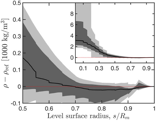 Figure 11. Same as Figure 9 but background density derived from adiabat calculated for Z=0.1 and Z=0.135.
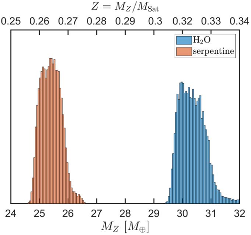 Figure 10. Residual mass in heavy elements and corresponding residual bulk metallicity assuming either pure H2O ice or pure serpentine rock EOS. These are end-members of what is likely a mixture of both materials in unknown ratio. The figure shows the mass in heavy elements inferred with a reference density based on a H/He adiabat with Z=0.275 extending throughout the planet. It should be interpreted as an upper bound for adiabatic models, as it excludes the possibility of a pure heavy-element core.
 Figure 9. Residual density above a background derived from a reference adiabat calculated for a H/He mixture with He mass fraction Z=0.275 and ( ) =T 1 bar 140 K . The thick curve is the sample median, and the dark and light shaded regions include 68% and 96% of the sample, respectively.
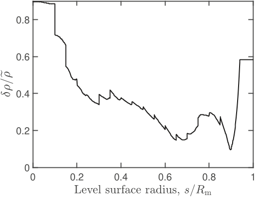 Figure 4. Width of the distribution of density values found in the posterior sample at each radius. The quantity dr is the difference of 84th and 16th percentile values, giving the equivalent of a 2σ spread; r is the sample median density. The flat region near =s R 1m is a consequence of the relatively strong prior imposed in that region (see Appendix C).
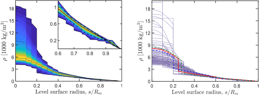 Figure 3. Visualization of the posterior probability distribution of Saturn interior density profiles. Left: the thick black line is the sample median of density on each level surface. The dashed lines mark the the 16th and 84th percentiles, and the dotted lines mark the 2nd and 98th percentiles; between the lines, the percentile value is indicated by color. Right: several hundred profiles covering the sampled range. By nature of the MCMC algorithm, regions of the figure where lines are closer together correspond to high-likelihood areas of parameter space. For comparison, three profiles derived by physical models with a pure H2O core (Mankovich et al. 2019, same profiles as in Figure 2) are overlaid.
 Figure 18. Gravitational harmonics of the empirical models of Figure 3 of the main text. The coefficients for Saturn’s observed gravity (Iess et al. 2019) are indicated by a red circle.
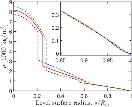 Figure 2. Three representative Saturn density profiles from M19. These profiles were derived using the standard, three-layer assumption, and thus represent only a subset of possible profiles. On the other hand, they are known to be in strict agreement (by construction) with theoretical EOSs throughout the interior. The inset shows a zoomed-in view of the top part of the envelope. The red solid line is the same curve as in the full-scale figure; the black dotted line is a quadratic fit, a good approximation of the upper envelope overall, and the blue dashed line is a quartic fit to the segment >s R 0.94m , a much better fit there (Appendix A).


