
All figures (9)

Figure 2: (a) Shows a Daubechies wavelet analysis of DDoS traffic data while (b) presents the denoised traffic residuals. 14 
Table 1: Example sound files 
Figure 1: (a) shows a Daubechies wavelet analysis of normal traffic data while (b) shows the denoised traffic residuals. 13 
Figure 5: This screen grab shows the double spike in the sent bytes and received bytes variables. The log returns are negative jumps as shown by the descending peaks. The sound files spike2 1s a.wav and spike2 1s.wav demonstrate how this sounds at playback speeds of 1 s per record, using the absolute and signed log returns respectively. spike2 20ms a.wav is the same traffic segment but played back at 20 ms per record and using absolute (unsigned) values. 
Figure 6: This screen grab shows shows a series of spikes in the sent bytes and received bytes variables.The audio file multiSpike 1s.wav demonstrates how this sounds at a playback speed of 1 s per record using signed log return values. There is an audible difference between the positive and negative traffic changes. However, notice how the peaks are not salient when playing back signed values at the faster rate of 20 ms as in multiSpike 20ms.wav — the peaks occur at around the 1.5 s mark in the audio file. 
Figure 8: This screen shot of the voice channel section shows log return spikes occurring on all four channels with the largest values occuring in the sent bytes and sent packets streams. These spikes generate a noticeable increase in the amplitude and brightening of the timbre of the soundscape. 
Figure 7: This screen grab shows the same series of spikes as Fig 6 but this time using the unsigned log returns. The sound files multiSpike 1s a.wav and multiSpike 20ms a.wav are recordings of this traffic segment played back at 1 s and 20 ms per record respectively. In both cases the traffic peaks are quite noticeable. The file multiSpike 20ms as.wav demonstrates how squaring the log return values leads to an even more marked effect. 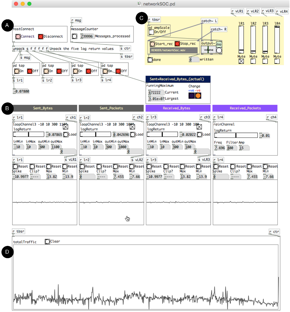
Figure 4: The socs application. Section A deals with reading the network traffic from the capture device. Section B contains the voice definitions to which each traffic variable is mapped. Section C is a mixer to convert the four separate audio streams into a single stereo feed. Section D is a graphical display of the combined variables being monitored. The channel graph plots are updated more frequently than the aggregate graph plot. 
Figure 3: Schematic view of the SOC sonification system for four network traffic variables: number of bytes sent (bs), number of packets sent (ps), number of bytes received (br), number of packets received (pr).


