
All figures (12)
 FIG. 4: Panel (a) shows the growth rate, γm, of type 2 SuperHMRI, optimized over a set of parameters (α, k∗z ,Ha ∗, Re∗), and represented as a function of Pm, at fixed Ro = 1.5. Panels (b) and (c) show the corresponding Ha∗m and Re ∗ m, respectively. For both Pm ≪ 1 and Pm ≫ 1, γm tends to constant values. The re-scaled Hartmann and Reynolds numbers vary as Ha∗m ∝ Pm −1/2 and Re∗m ∝ Pm −1 for Pm ≪ 1, and as Ha∗m ∝ Pm 1/3 and Re∗m ∝ Pm −1/4 for Pm ≫ 1. Panels (b) and (c) are compensated by these factors to more clearly highlight these scalings. The dashed lines are at Pmc1 = 0.223 and Pmc2 = 4.46, marking the Pm = O(1) region where no instability exists.
 FIG. 3: Imaginary part of the eigenvalues, that is, frequency ω = Im(γ), at small Pm = 10−6 (a) and large Pm = 100 (b) corresponding, respectively, to the growth rates shown in Figs. 1(a) and 2(a) at the same Ro = 1.5 (blue), Ro = 2 (green), Ro = 6(red) and α = 0.71. Dashed lines correspond to the frequency of inertial oscillations, ωio = 2α(1 + Ro) 1/2, for these parameters. Note that at small Pm the frequencies are positive, while at large Pm are negative (−Im(ω) is plotted in panel b), implying opposite propagation directions of the wave patterns at these magnetic Prandtl numbers.
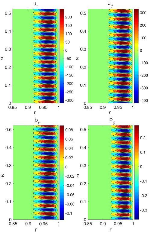 FIG. 10: Same as in Fig. 8, but for large Pm = 100 and conducting boundary conditions. The parameters (β,Ro,Ha,Re) are the same as in Fig. 7(b) and the axial wavenumber is kzm = 141, corresponding to the maximum growth rate (peak on the blue curve in that panel) for the given values of these parameters. For the sake of comparison of the eigenfunction structures and lengthscales with those at small Pm, the z-axis has the same range as in Figs. 8 and 9. At large Pm, the eigenfunctions in the presence of insulating boundaries are in fact identical to the ones for the conducting boundaries shown here at the same values of the main parameters and hence we do not plot those eigenfunctions.
 FIG. 8: Eigenfunctions of the radial and azimuthal velocity and magnetic field for type 2 Super-HMRI in the global case as a function of (r, z) at small Pm = 10−3, the narrow gap η̂ = 0.85 and conducting boundary conditions on the cylinders. The parameters (β,Ro,Ha,Re) are the same as those in Fig. 6(b) and the axial wavenumber is chosen to be kzm = 24, at which the growth rate for the given values of these parameters reaches a maximum (peak on the blue curve in that panel).
 FIG. 9: Same as in Fig. 8, but for insulating boundary conditions on the cylinders. The main parameters are again the same as in Fig. 6(b), but now the axial wavenumber is chosen to be kzm = 23, corresponding to the largest growth rate for the given values of these parameters (peak on the red curve in that panel) and the boundary conditions.
 FIG. 13: Growth rate of type 2 Super-HMRI vs. kz for a power-law radial profile of the angular velocity with Ro = 0.7 and a very narrow gap η̂ = 0.94, which are close to those of the solar tachocline. The boundary conditions are conducting at the inner and insulating at the outer walls, as often used in solar tachocline studies. The other parameters are taken also of the same order as those for the tachocline (see text): β = 500, Pm = 0.01, Ha = 2500 and Re = 1.5 · 106. As in Fig. 6, black dashed line shows the WKB result for these parameters, but at much higher radial wavenumber kr0 = π(1− η̂)−1 ≈ 52.4, corresponding to a narrower gap.
 FIG. 6: Growth rate, Re(γ) (panels (a), (b), (c)), and frequency, ω = Im(γ) (panels (d), (e), (f)), vs. kz in the global case with the narrow gap η̂ = 0.85 and power-law angular velocity profile with constant Ro = 3.5 < RoULL in the presence of conducting (blue) and insulating (red) boundary conditions imposed on the cylinders. In all panels, β = 100, Pm = 10−3, while (Ha,Re) = (2000, 2·106) in panels (a) and (d), (Ha,Re) = (2800, 3·106) in panels (b) and (e), and (Ha,Re) = (3200, 3.5·106) in panels (c) and (f). Black dashed curve in each panel is accordingly the growth rate or frequency resulting from the local WKB dispersion relation (Eq. 4) for the same values of the parameters corresponding to that panel and a fixed kr0 = π/δ, where δ = 1− η̂ is the gap width in units of ro. It is seen that in the local and global cases, the shape of the dispersion curves is qualitatively same, with comparable growth rates, frequencies and corresponding wavenumbers, however, the boundary conditions tend to shift the growth rates towards lower axial wavenumbers, while the frequencies towards larger wavenumbers relative to those in the local case. Also, insulating boundaries lower the growth rate about three times. As for the frequencies, they are close to each other for both these boundaries and smaller than those in the local case at a given kz.
 FIG. 11: Growth rate Re(γ) vs. kz for the TC flow with the wide gap, η̂ = 0.5, and the inner cylinder at rest. Panel (a) focuses on Pm ≪ 1, with solid lines having fixed β = 1, S = 4 and Rm = 20 but different Pm, dot-dashed line β = 2, S = 8, Rm = 80, Pm = 10−5, and dashed line β = 3, S = 12, Rm = 180, Pm = 10−5. Panel (b) focuses on Pm ≫ 1, with solid lines having fixed β = 1, Ha = 1600 and Re = 8 · 104 but different Pm, dot-dashed line β = 0.4, Ha = 640, Re = 1.28 · 104, Pm = 500, and dashed line β = 0.5, Ha = 800, Re = 2 · 104, Pm = 500.
 FIG. 12: Growth rate for the TC flow with the positive shear and wide gap, maximized over kz and represented in (S,Rm)plane, at fixed Pm = 10−6 and β = 1. As in the local equivalent (Fig. 1(c)), the unstable region is localized in (S,Rm)plane, reaching a maximum at Sm = 5.2 and Rmm = 25.
 FIG. 7: Same as in Fig. 6, but at large Pm = 100 with (Ha,Re) = (200, 2000) in panels (a) and (d), (Ha,Re) = (400, 4000) in panels (b) and (e), and (Ha,Re) = (800, 8000) in panels (c) and (f). Note that in this case the growth rates and frequencies (plotted is −ω = −Im(γ)) are nearly indistinguishable for conducting and insulating boundary conditions, in contrast to the small-Pm regime depicted in Fig. 6. Black dashed curve in each panel is again accordingly the growth rate or frequency resulting from the WKB dispersion relation (Eq. 4) with kr0 = π/δ and the same values of the parameters corresponding to that panel. For the growth rate, the difference between the local and global dispersion curves increases with increasing Hartmann and Reynolds numbers mainly at smaller kz . 10 (panel (c)), whereas for the frequencies these curves are quite close to each other. Overall, the agreement between the WKB and 1D analysis at these large Pm = 100 is much better than that at small Pm = 10−3 in Fig. 6.
 FIG. 1: Panel (a) shows the growth rate Re(γ) vs. k∗z at fixed Ha∗ = 90, Re∗ = 8 · 103, α = 0.71 (i.e., k∗r = k ∗ z ) and Pm = 10−6 for different Ro = 1.5 (blue), 2 (green), 6 (red). New type 2 Super-HMRI branch exists at smaller k∗z and finite Pm, for all three Ro values. By contrast, type 1 Super-HMRI branch at larger k∗z appears only for Ro = 6 > RoULL from these there values of the Rossby number, but persists also in the inductionless limit (Eq. 5, dashed-black line). For the same Pm, panel (b) shows the growth rate of type 2 SuperHMRI, maximized over a set of the parameters (k∗z , Ha ∗, Re∗) and normalized by Ro1.75, vs. α, while panel (c) shows the growth rate, maximized over k∗z and α, as a function of Ha∗ and Re∗ at Ro = 1.5 and the same Pm = 10−6.
 FIG. 2: Same as in Fig. 1, but at Ha∗ = 5, Re∗ = 0.1, α = 0.71 in panel (a) and Pm = 100 in all panels. New type 2 Super-HMRI branch exists at higher k∗z than those at small Pm, while type 1 Super-HMRI branch is absent. In panel (b), the maximum growth rate now exhibits the scaling with Rossby number, Ro1.18, different from that at small Pm. In panel (c), the maximum growth occurs now at orders of magnitude smaller Ha∗m and Re ∗ m than those at small Pm in Fig. 1(c) at the same Ro = 1.5.


