
All figures (11)
 Figure 4. Vertical distribution of particles loosely coupled to the gas (τΩ> 1, corresponding to large particles). The dashed line shows the expected distribution for particles tightly coupled to the gas, neglecting oscillations, while the dotted line shows the analytical model for particles loosely coupled to the gas (see Equation (23)), which shows an excellent agreement with LIDT3D. Note that the particle’s scale height diminishes with the particle’s stopping time in agreement with Youdin & Lithwick (2007).
 Figure 11. Example of the trajectory of a 10 cm grain. Top: path in the R/Z plane; bottom: temperature of the gas surrounding the particle as a function of time.
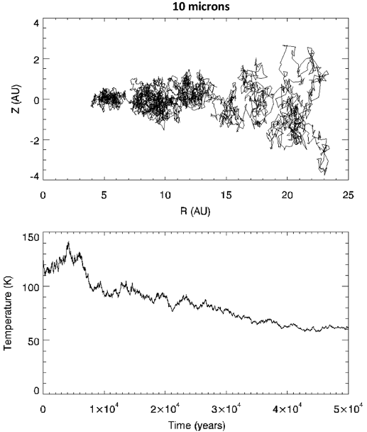 Figure 10. Example of the trajectory of a 10 μm particle. Top: path in the R/Z plane; bottom: temperature of the gas surrounding the particle as a function of time.
 Figure 9. Example of the trajectory of a 1 μm particle. Top: path in the R/Z plane; bottom: temperature of the gas surrounding the particle as a function of time. When the particle falls below 0.5 AU (∼33,000 yr here), it is eliminated from the disk.
 Figure 1. Test of 1D particle diffusion of a solute (particles) in a solvent (gas) with (panels (b) and (d) and without (panels (a), (c)) corrections for the density of the solvent. Top row: the solid line shows the number of particles in each X bin of the simulation; the dashed line shows the region where all particles were initially released. Bottom row: density of particles (number of particles in each X bin divided by the local gas density). The solid histogram shows the particles, the dashed line shows the initial state, and the solid sinus curve shows the absolute density of the gas. Left column: without using the density corrections, right column: using the density correction.
 Figure 3. Vertical dust density distribution obtained with a constant diffusion coefficient for different-sized particles after 1000 yr of evolution at 1 AU. Solid line: particle distribution obtained with the LIDT3D code; dashed line: analytical model for small particles tightly coupled to the gas (Equation (22)). In each graph, the title reports τΩ (i.e., the particle stopping time times the local Keplerian frequency), which is roughly the Stokes number. Note the excellent agreement that is obtained for τΩk < 0.2. For larger values of τΩk the analytical model for particles tightly coupled to the gas fails. The case of big particles is presented in Figure 4.
 Figure 8. Comparison of midplane and 3D diffusion. This figure displays the surface density of particles as a function of the distance to the star at four different epochs. The disk has a surface density decreasing as r−1 and α = 0.01. Solid line: 3D simulation; dashed line: 2D simulation in which particles are confined to the disk’s midplane. The particle’s radius is 0.1 μm.
 Figure 7. Example of diffusion at 10 AU in the (R, Z) plane. Five thousand particles of different sizes (see color scale on the right) were released at 10 AU. For 500 yr they do not evolve radially in order to reach a vertical steady state. Then they are allowed to evolve freely in the turbulent gas disk. In panels (a)–(d) the (R, Z) location of all particles is displayed. The solid line shows the pressure scale height. Here the Schmidt number is taken from Youdin & Lithwick (2007). Note that radial diffusion is more efficient at higher values of Z/H. In panel (e) the particle–gas coupling parameter, Ωτ (∼Stokes number), is displayed as a function of Z at 10 AU, and for different particle sizes.
 Figure 5. Test of radial diffusion. Ten thousand particles were released at 10 AU initially, with a 0.1 μm radius. They are forced to evolve in the midplane only of a gaseous disk with a gas surface density decreasing as r−1. These plots show the dust surface density after 2500 and 5000 yr (top) and 10,000 and 15,000 yr (bottom) evolution. For comparison, the surface density obtained from the explicit integration of the 1D hydrodynamical diffusion Equation (23) is shown in black and shows excellent agreement with the results of LIDT3D.
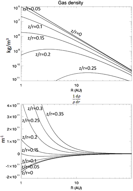 Figure 6. Top: gas density in a disk with a surface density decreasing as r−1 for different values of Z/R. Note that the steepest gradient is in the midplane (Z/R = 0). Bottom: corresponding values of 1/ρg × grad(ρg), which give the net direction of the local diffusive flux. Note that in the midplane (Z/R = 0) the diffusive flux is always negative (i.e., directed inward), whereas above the midplane, for Z/R > 0.15 the diffusive flux can be positive (i.e., directed outward).
 Figure 2. Location of 10,000 different-sized particles (color-to-size correspondence is given on the right scale) after 10,000 yr evolution at 1 AU. A constant diffusion coefficient was used. We clearly see the sedimentation process: small particles are widely spread vertically, whereas big particles sediment rapidly and gather close to the midplane (z = 0). The solid horizontal lines show the location of the pressure scale height.


