
All figures (23)
 Fig. 1. Sketch of the Lagrangian-Eulerian mapping relating a material Lagrangian point X at t = 0 and a spatial Eulerian one x at t > 0 through Φ, and its Jacobian F(X, t) = ∂Φ
 Fig. 14. Twisting column — Time evolution of non-dimensionalised height of the column measured at initial point xT = (0, 0, 6) (left) — Numerical dissipation (88) of second order scheme (center) — Percentage of bad cells detected at each time step (right).
 Fig. 9. Cantilever thick beam — Comparison between the MOOD cascades: P1 → P0 (LAM P0-lim) and P1 → Plim1 → P0 (LAM P1-lim) for the computed numerical dissipation (88) as a function of time (left) and percentage of bad cells detected at each time step (right).
 Fig. 19. L-shaped block test problem — From top-left to bottom-right: time t = 2.5, 5.0, 7.5, 10.0, 12.5 and 15 s.
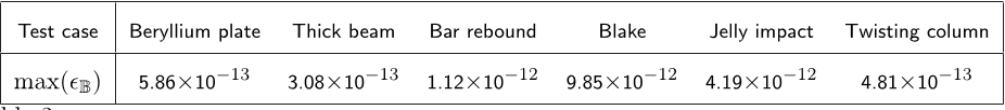 Table 3 Maximal value of B for the first 75000 time-steps of the 2D and 3D tests cases in this paper.
 Fig. 20. L-shaped block test problem — Angular momentum Ac in x (green), y (red) and z (blue) directions as a function of time.
![Fig. 10. Blake’s problem — Computational mesh of the needle domain ω = [r, θ, φ] = [0.9, π/180, π/180] with h = 1/1000 (left) and pressure distribution at the final time tfinal = 1.6 · 10−4 s (right).](/figures/fig-10-blakes-problem-computational-mesh-of-the-needle-3no5wx1y.png) Fig. 10. Blake’s problem — Computational mesh of the needle domain ω = [r, θ, φ] = [0.9, π/180, π/180] with h = 1/1000 (left) and pressure distribution at the final time tfinal = 1.6 · 10−4 s (right).
Fig. 10. Blake’s problem — Computational mesh of the needle domain ω = [r, θ, φ] = [0.9, π/180, π/180] with h = 1/1000 (left) and pressure distribution at the final time tfinal = 1.6 · 10−4 s (right). Table 2 Numerical errors in L2 norm and convergence rates for the 2D swinging plate test computed with second order of accuracy Lagrange ADER scheme at time tfinal = π/ω. The error norms refer to the variables u (horizontal velocity), B11 (first component of the left Cauchy-Green tensor B) and T11 (first component of the Cauchy stress tensor T).
 Fig. 13. Twisting column — Beam shape and pressure distribution at output times t = 0.00375, t = 0.075, t = 0.1125, t = 0.15, t = 0.1875, t = 0.225, t = 0.2625 and t = 0.3 (from top left to bottom right). The shape is compared with respect to the initial configuration (hollow box).
 Fig. 4. Left: Split of a tetrahedron into sub-tetrahedra by inserting six new midpoint edge vertices to get four corner sub-tetrahedra (colored ones). After choosing a diagonal (yellow line) to split the remaining central octahedron into fours more sub-tetrahedra, it yields a total of eight sub-tetrahedra — Right: example of 2D partitioning on NCPU = 4 threads (colors), the refinement is performed locally to each thread, only the coarse partition of large black triangles is actually built across the threads.
 Fig. 5. Sketch for the elastic vibration of a beryllium plate in section 5.2 (left) and the finite deformation of a cantilever thick beam in section 5.3 (right).
 Fig. 6. Elastic vibration of a beryllium plate — Numerical results at output times t = 10−5 (top), t = 2 · 10−5 (middle) and t = 3 · 10−5 (bottom) for pressure (left) and cell order map (right), the cells in yellow are at unlimited order 2, while the blue ones are the BJ limited ones. No first-order updated cell is observed.
 Fig. 18. Impact of a jelly droplet — Time evolution of the maximum spreading of the droplet L/L0 in the case neo-Hookean model (a = −1, black line) or non-linear one (a = 0, red line) — The impact velocity is 2 m.s−1 (left) and 3 m.s−1 (right).
 Fig. 16. Rebound of a hollow circular bar — Time evolution of vertical displacement of the points on the top plane xT = (1.6, 0, 32.4) · 10−3m and on the bottom plane xB = (1.6, 0, 4) · 10−3m (left) and percentage of bad cells detected at each time step (right).
 Fig. 17. Impact of a jelly droplet with impact velocity 3 m.s−1 — Time evolution of the droplet shape at different output times for neo-Hookean model (a = −1, petroleum shade) or non-linear one (a = 0, black shade).
 Fig. 11. Blake’s problem— Mesh convergence of the second order solution towards the reference solution (red) for the radial pressure (top row) and radial deviatoric stress (bottom row) at time tfinal = 1.6 · 10−4 (left) and zoom across the shock (right). Remind that LAM P1-lim corresponds to cascade: P1 → Plim1 → P0.
 Fig. 7. Elastic vibration of a beryllium plate — Comparison between the MOOD cascades: P1 → P0 (LAM P0-lim) and P1 → Plim1 → P0 (LAM P1-lim) for the vertical displacement at the barycenter of the plate (left) and the computed numerical dissipation (88) as a function of time (right).
 Table 1 Strong scaling computed for the L-shaped block test case presented in section 5.8.The computational time needed to perform an element update with second order of accuracy in space and time is addressed with τEU .
 Fig. 15. Rebound of a hollow circular bar — Time evolution of the deformation and pressure distribution at output times at times t = 50 µs then 75, 100, 125, 150, 200, 300 and the final time t = 325 µs (from top left to bottom right).
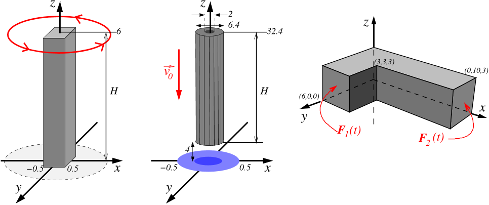 Fig. 12. Sketch for the twisting column in section 5.5 (left) and the rebound of a hollow circular bar from section 5.6 (middle), and, L-shaped block test problem from section 5.8 (right).
 Fig. 8. Cantilever thick beam test case — Pressure distribution with deformed shapes (left column) and cell order map (right column) with the second-order a posteriori limited Lagrangian scheme at output times t = 0.375, t = 0.75, t = 1.125 and t = 1.5 (from top to bottom row) — Comparison of the deformed shape computed using the simpler cascade P1 → P0 in black line on the left panels only.
 Fig. 3. Sketch of the current Lagrangian numerical method and its associated MOOD loop.
 Fig. 2. Left: Reference simplicial element ωe in coordinates ξ = (ξ, η, ζ) — Right: cell ωc, subcell ωpc and geometrical face/cell/point centers and outward pointing face normal nf to each face f .


![Fig. 10. Blake’s problem — Computational mesh of the needle domain ω = [r, θ, φ] = [0.9, π/180, π/180] with h = 1/1000 (left) and pressure distribution at the final time tfinal = 1.6 · 10−4 s (right).](/figures/fig-10-blakes-problem-computational-mesh-of-the-needle-3no5wx1y.webp)


