
All figures (13)
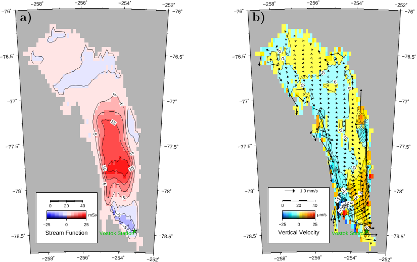 Fig. 2. Water depth and potential temperature dependence of isopycnals (Feistel, 2003; Jackett et al., 2006). The black solidus line shows the depth-dependent freezing point of fresh water (Feistel, 2003; Jackett et al., 2006), the red solidus line indicates the linearized form of the freezing point equation adjusted for Lake Vostok. The dashed line connects the isopycnal’s vertices and indicates the line of maximum density (LoMD). The dotted gray line indicates the former LoMD according to Haidvogel and Beckmann (1999) as published in Thoma et al. (2008b). Coloured dots show the captured space of potential temperatures and equivalent water depth for Lake Vostok, Lake Concordia, and Lake Ellsworth, respectively. Dots within the grey shaded area above the solidus line represent supercooled water masses with freezing capability.
 Fig. 4. a) Zonal and meridional overturning stream functions (1mSv = 103 m3/s). b) South-north temperature cross section across Lake Vostok along the track indicated in Figure 1 and 3b.
 Fig. 5. Modelled accreted ice thickness (in meter) at the ice–lake interface The corresponding ice flow direction is indicated. The horizontal flow velocity is assumed to be 3.7m/a, which results in 210m of accreted ice, as measured at Vostok Station. This value is within the proposed measured velocities of about 1.9 and 4.2 m/a (e.g., Kwok et al., 2000; Bell et al., 2002; Tikku et al., 2004; Wendt, 2005).
 Fig. 3. a) Modelled basal mass balance at the ice–lake interface. Negative values (blue/green) indicate melting, positive (yellow/red) values freezing. Velocities in the ice–lake boundary layer are indicated by arrows. b) Modelled temperatures at the ice–lake interface. The solid red line indicates the track along the cross sections shown in Figures 4b.
 Fig. 2. Water depth and potential temperature dependence of isopycnals (Feistel, 2003; Jackett et al., 2006). The black solidus line shows the depth-dependent freezing point of fresh water (Feistel, 2003; Jackett et al., 2006), the red solidus line indicates the linearized form of the freezing point equation adjusted for Lake Vostok. The dashed line connects the isopycnal’s vertices and indicates the line of maximum density (LoMD). The dotted gray line indicates the former LoMD according to Haidvogel and Beckmann (1999) as published in Thoma et al. (2008b). Coloured dots show the captured space of potential temperatures and equivalent water depth for Lake Vostok, Lake Concordia, and Lake Ellsworth, respectively. Dots within the grey shaded area above the solidus line represent supercooled water masses with freezing capability.
 Fig. 10. Modelled accreted ice thickness (in meter) at the ice–lake interface The corresponding ice flow line direction is east-northeastward. The horizontal ice flow velocity is assumed to be 25 cm/a (Tikku et al., 2005).
 Fig. 9. a) Zonal and meridional overturning stream functions (1 Sv = 10m3/s). b) South-north temperature cross section across Lake Concordia along the track indicated in Figure 6 and 8b.
 Fig. 1. Bedrock topography (a) and water column thickness (b) of Lake Vostok. The solid red line indicates the track along the cross sections shown in Figures 4b.
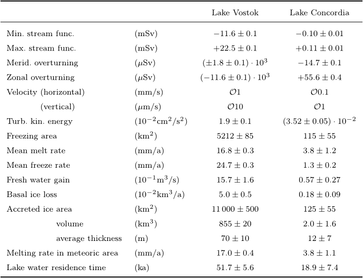 Table 1 Revised values for important modelled results within subglacial lakes with respect to improved versions of the EoS and the EoFP. The uncertainties are derived from model runs with varying boundary conditions.
 Fig. 1. Bedrock topography (a) and water column thickness (b) of Lake Vostok. The solid red line indicates the track along the cross sections shown in Figures 4b.
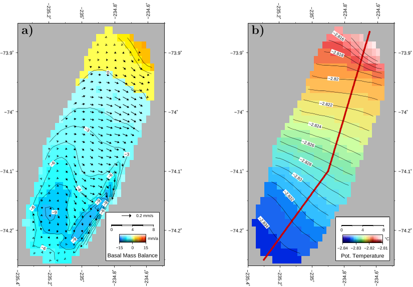 Fig. 8. a) Modelled basal mass balance at the ice–lake interface. Negative values (blue/green) indicate melting, positive (yellow/red) values freezing. Velocities in the ice–lake boundary layer are indicated by arrows. b) Modelled temperatures at the ice–lake interface. The solid red line indicates the track along the cross sections shown in Figures 9b.
 Fig. 7. a) Vertically integrated mass transport stream function (1 Sv = 10m3/s). b) Integrated vertical velocity, arrows indicate the flow in the lake’s bottom layer.
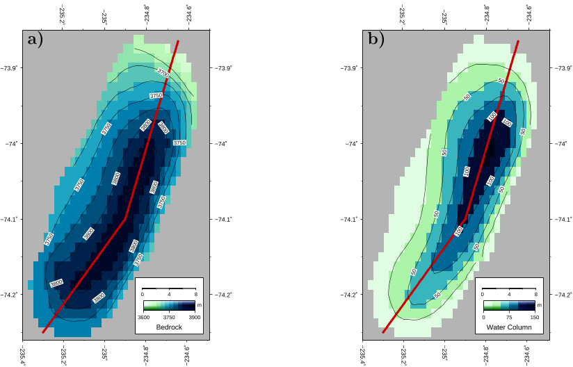 Fig. 6. Bedrock topography (a) and water column thickness (b) of Lake Concordia. The solid red line indicates the track along the cross sections shown in Figures 9b.


