
All figures (13)
 Figure 8: Left (a, c, e): The mean zonal profiles of Convergence of Momentum Transport. Right (b, d, f): Northward Heat Transport (b, d, f). The x axis indicates the jth CLV. In (a, c, e) the solid lines indicate the sign switch of the barotropic conversion CBT from positive to negative. In (b, d, f) the dash-dotted lines indicate the sign switch of the baroclinic conversion CBC from positive to negative. The black dotted lines show the CLV with smallest positive LE. The y axis shows the distribution in the meridional direction in 103km.
 Table 3: Transports and Conversions - The conversion is positive if the correlation between gradient of the background state and eddy transport of the CLVs is negative. Note that for CPK the baroclinic stream function ψT is proportional to the vertical gradient of the stream function.
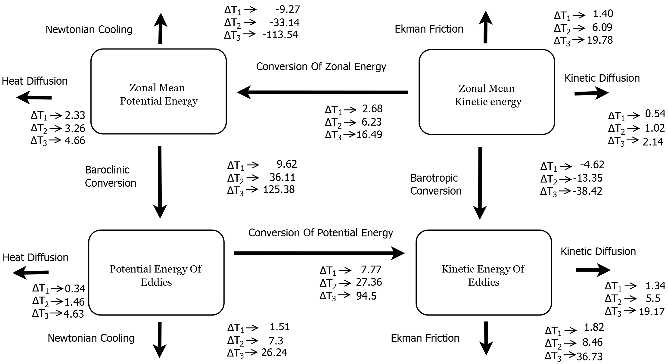 Figure 3: Flow Chart of the Lorenz Energy Cycle for three ∆T (Units of Conversions are 105m2/s3). The arrows indicate the average sign of the energy conversions, sinks and sources of the zonal and eddy energies. For every temperature gradient (∆T1 = 39.81K, ∆T2 = 49.77K and ∆T3 = 66.36K) the dominant source of energy is Newtonian cooling, which inputs energy to the zonal mean potential energy. The important conversions are the baroclinic conversion which is related to the northward heat transport (see fig. 2 c) and the barotropic conversion related to the center pointed momentum transport (see fig. 2 d). The main energy losses occour by converting the potential energy of the eddies into kinetic energy, where it is lost mainly due to kinetic diffusion and Ekman friction. We observe an intensification of the cycle for a larger meridional temperature gradient ∆T .
 Figure 10: The panels show the average correlation (solid lines) of the subspaces spanned by the n fastest growing CLVs (a) and the n fastest decaying CLVs (b) with the considered trajectories of ∆T (dotted: 39.81K , dashed: 49.77K, solid: 66.36K). The parameter n is indicated on the x axis. The average is done over the mean correlation for different reference points of the CLVs (41 reference points, equally distributed over a 12 years period). The corresponding σ area is indicated by the shaded regions. The vertical dashed dotted lines indicate where the expansion includes exactly all baroclinically unstable CLVs (Panel a) or all baroclinically stable CLVs (Panel b). Panel b) also shows the expansion into a randomly chosen basis (almost diagonal dashed lines). The comparison of both panels shows the higher explanatory power of CLVs with a higher LE.
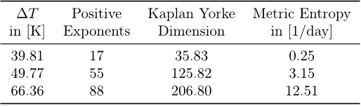 Table 2: Properties of the attractor
![Figure 5: Lyapunov Exponents [1/day] for three meridional temperature gradients (dotted: 39.81K , dashed: 49.77K, solid: 66.36K)](/figures/figure-5-lyapunov-exponents-1-day-for-three-meridional-3dgh142r.png) Figure 5: Lyapunov Exponents [1/day] for three meridional temperature gradients (dotted: 39.81K , dashed: 49.77K, solid: 66.36K)
Figure 5: Lyapunov Exponents [1/day] for three meridional temperature gradients (dotted: 39.81K , dashed: 49.77K, solid: 66.36K) Table 1: Parameters and Variables used in this model and the respective adimensionalization scheme. Not that the scales for time and length are t = 104s = 1/f0 and L = 107 π m
 Figure 6: Left Side: The three figures show the dependence of the inputs and the conversion of the Lorenz energy cycle on the corresponding Lyapunov exponent for each of the three meridional temperature gradients (dotted: 39.81K , dashed: 49.77K, solid: 66.36K). The magnified view (right side) shows the CLVs with near zero growth rate including the corresponding average eddy observables from the classical Lorenz energy cycle (gray horizontal lines). The y axis units are in 1/day.
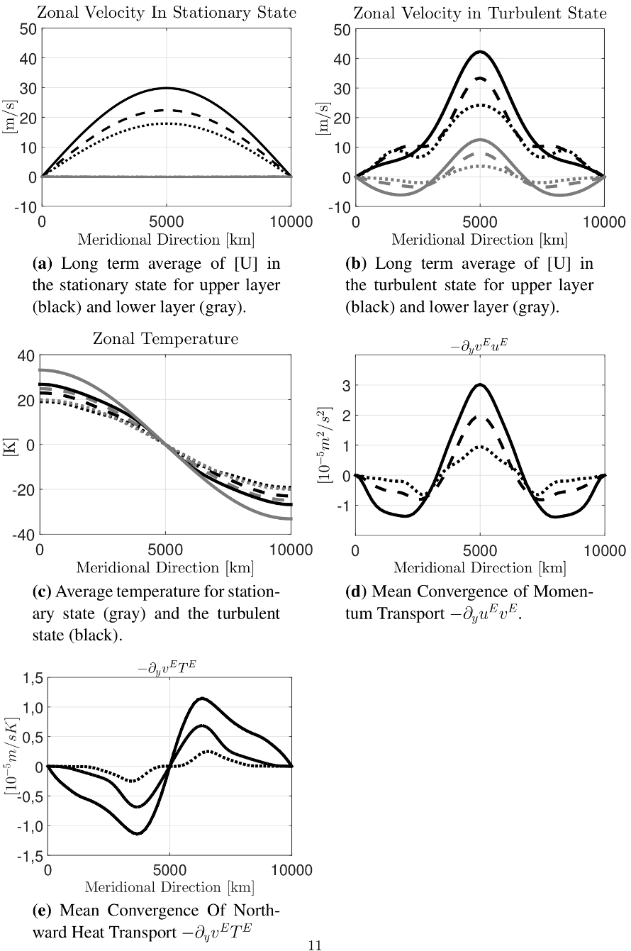 Figure 2: The mean state of the trajectory (averaged over a period of 25 years) for the three forced meridional temperature gradients ∆T (dotted: 39.81K , dashed: 49.77K, solid: 66.36K). The superscript E indicates the eddy terms.
 Figure 4: The graphs show the modulus of the average correlation <ψ B ,ψ′> ||ψB ||||ψ′|| between the background state and the CLVs, where the bilinear product < ·, · > is defined via the kinetic, potential and total energy. The grey shaded areas are the 3 σ confidence intervals. We estimated the effective number of degrees of freedom by dividing the time series into blocks corresponding to the e folding time of the autocorrelation function (Leith, 1973). The x axis indexes the CLVs. Similar results have been obtained for non zonal stationary states (Niehaus, 1981)
 Figure 1: These snapshots show the streamfunction fields for the upper and lower layer. The upper is on the left side and the lower layer is found on the right side. Note, that in order to use a grey scale, the scale of the colorbars is different in every panel. The flow shows a clearly baroclinically unstable and barotropically stable configuration (see section 4)
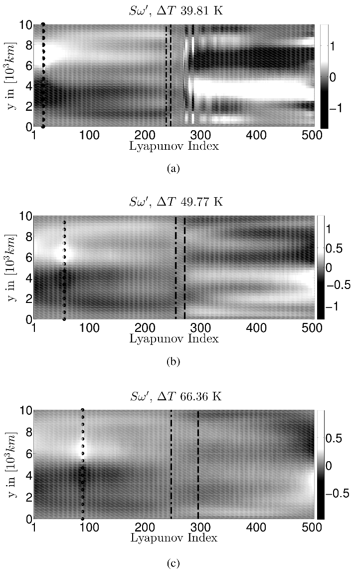 Figure 9: The mean zonal profiles of the conversion of heat S? for the three meridional temperature gradients plotted for every CLV ((a) ∆T = 39.81 K, (b) ∆T = 49.77 K and (c) ∆T = 66.36 K). The black vertical dashdotted lines indicate the change of sign from positive to negative of the baroclinic conversion CBC. The dashed lines indicate the change of sign in the conversion from potential to kinetic energy CPK. The black dotted lines show the CLV with the smallest positive LE. The y-axis shows the distribution in the meridional direction in units of 103 km. The x-axis indicates the jth CLV. 25
 Figure 7: Left Side: The four figures show the dependence of the different sinks of the Lorenz energy cycle on the corresponding Lyapunov exponent for each of the three meridional temperature gradients (dotted: 39.81K , dashed: 49.77K, solid: 66.36K). The magnified view (right side) shows the CLVs with near zero growth rate including the corresponding average eddy observables from the classical Lorenz energy cycle (gray horizontal lines). The y axis units are in 1/day.


![Figure 5: Lyapunov Exponents [1/day] for three meridional temperature gradients (dotted: 39.81K , dashed: 49.77K, solid: 66.36K)](/figures/figure-5-lyapunov-exponents-1-day-for-three-meridional-3dgh142r.webp)


