
All figures (25)
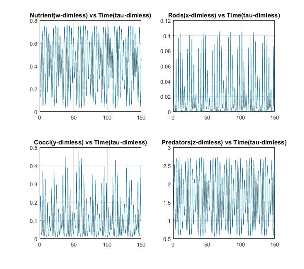 Figure 3.1. Plots of the four dimensionless variables w (nutrient), x (rods), y (cocci) and z (predators). Chaotic dynamics is evident.
 Table 4.1. Values for Shannon’s measures of uncertainty (SMU) and the resulting redundancy (RD) values for the discrete probability distributions shown in Figures 4.1 through 4.4. The maximum possible SMU = (29)1/2 = 4.392.
![Figure 2.3. 3-D system space plots of Equations (4) solution with an inflowing nutrient concentration given by Dn0 = [0.15(1 - 0.5sin(0.52t))]. A strange attractor is evident.](/figures/figure-2-3-3-d-system-space-plots-of-equations-4-solution-2i9a6qsj.png) Figure 2.3. 3-D system space plots of Equations (4) solution with an inflowing nutrient concentration given by Dn0 = [0.15(1 - 0.5sin(0.52t))]. A strange attractor is evident.
Figure 2.3. 3-D system space plots of Equations (4) solution with an inflowing nutrient concentration given by Dn0 = [0.15(1 - 0.5sin(0.52t))]. A strange attractor is evident. Table 1.1. Parameter values used in Equations (1.10) that yield chaotic dynamics with the dilution rate utilized in Becks et al. (2005).
![Figure 1.6. Simulated nutrient and microbe dynamics that match the Becks et al. [2005, Fig. 1] results for D = 0.9/d (0.0375/hr).](/figures/figure-1-6-simulated-nutrient-and-microbe-dynamics-that-3u6k06k2.png) Figure 1.6. Simulated nutrient and microbe dynamics that match the Becks et al. [2005, Fig. 1] results for D = 0.9/d (0.0375/hr).
Figure 1.6. Simulated nutrient and microbe dynamics that match the Becks et al. [2005, Fig. 1] results for D = 0.9/d (0.0375/hr). Figure 3.2. A system-space plot of dimensionless rods vs. cocci vs. predators yields the usual 3-D section of the 4-D strange attractor.
 Figure 1.1. Diagram of the Becks et al. (2005) chemostat system. A nutrient solution flowing left to right was consumed by two microbes (rods and cocci), with rods being stronger competitors for nutrient than cocci. A ciliate predator fed on both microbes, but preferred rods over cocci.
 Figure 1.7. Resulting nutrient and microbe dynamics with D = 0.75/d (0.03125/h). Both the model and experiments produced classical steady states, but all microbes survived in the experiments while the rods died out in the model.
 Figure 4.1. Discrete probability distribution for the dimensionless predator values shown in Figure 3.1. The domain of values was divided into 21 ranges of equal width 1.085E-1.
 Table 2.2. New parameters in Equations (2.1), and a set of test values. Units of “S” are mg-1, units of the specific death rates “δ” are hr-1, and 0 ≤ EF ≤ 1 is dimensionless.
 Table 1.2. Lyapunov exponents used to identify the presence of deterministic chaos based on the time series of concentrations shown in Figure 1.3 (Calculations were conducted using the R package “fractal” version: 2.0-1.)
 Figure 3.5. Dimensionless plot of predator cells (y-axis) vs. rod cells (x-axis). Again, the relationship is not random in the classical sense.
 Figure 4.2. Discrete probability distribution for the dimensionless nutrient values shown in Figure 3.1. The domain of values was divided into 21 ranges of equal width 3.6525E-2.
 Table 2.3. Diagnostic nonlinear dynamics parameters used to identify the presence of deterministic chaos based on the time series of concentrations shown in Figures 2.2 and 2.3. (Note: Analysis using R software packages “FRACTAL”).
 Figure 3.4. Dimensionless plot of predator cells (y-axis) vs. cocci cells (x-axis). Clearly, the relationship is not random in the classical sense.
 Figure 1.4. Resulting nutrient and microbe kinetics with D = 0.45/d (0.01875/hr.), as was done in the Becks et al. (2005) experiments.
 Figure 3.6. Dimensionless plot of Cocci cells (y-axis) vs. rods (x-axis). Again, the relationship is not random in the classical sense
 Figure 4.3. Discrete probability distribution for the dimensionless cocci values shown in Figure 3.1. The domain of values was divided into 21 ranges of equal width 2.35E-2.
![Figure 1.3. Irregular, non-periodic, dynamics of n(t), r(t), c(t) and p(t) associated with the system-space plot in Fig 1.2. By counting apparent concentration peaks, the mean frequency of the simulated data appears lower than that observed in Becks et al. [2005], but still within 50%. However, the mean model frequency can be selected by changing the dimensionless ratios of max specific growth and death rates to D (Chapter 3).](/figures/figure-1-3-irregular-non-periodic-dynamics-of-n-t-r-t-c-t-l20dtjr7.png) Figure 1.3. Irregular, non-periodic, dynamics of n(t), r(t), c(t) and p(t) associated with the system-space plot in Fig 1.2. By counting apparent concentration peaks, the mean frequency of the simulated data appears lower than that observed in Becks et al. [2005], but still within 50%. However, the mean model frequency can be selected by changing the dimensionless ratios of max specific growth and death rates to D (Chapter 3).
Figure 1.3. Irregular, non-periodic, dynamics of n(t), r(t), c(t) and p(t) associated with the system-space plot in Fig 1.2. By counting apparent concentration peaks, the mean frequency of the simulated data appears lower than that observed in Becks et al. [2005], but still within 50%. However, the mean model frequency can be selected by changing the dimensionless ratios of max specific growth and death rates to D (Chapter 3). Table 2.1. Parameter values selected for an initial mathematical analysis of the Becks et al. experiments using the generalized Kot et al. Model (2.1). Units for “μ” are hr-1, for “K” are mg/cc, and “Y” are mg/mg. Microbial masses are held constant at the values given (mg) in Chapter 1.
 Figure 2.2. Plots of nutrient and microbes as functions of time resulting from a solution of Equations (2.2), using parameter values specified in Tables 2.1 and 2.2, along with a sinusoidal, 12 hr. period, feeding rate. The only parameter difference with the solution shown in Figure 2.1 is the sinusoidal feeding rate.
 Figure 1.5. Resulting nutrient and microbe kinetics with D = 0.9/d (0.0375/hr).
 Figure 3.3. Dimensionless system-space 3-D section plot of nutrient vs. rods vs. predators.
 Figure 1.2. System-space (phase-space) plot of r(t), c(t) and p(t) for the parameters listed in Table 1.1 for D = 0.5/d (0.0208/hr) . A strange attractor is evident.
 Figure 4.4. Discrete probability distribution for the dimensionless rod values shown in Figure 3.1. The domain of values was divided into 21 ranges of equal width 5.3625E-3.


![Figure 2.3. 3-D system space plots of Equations (4) solution with an inflowing nutrient concentration given by Dn0 = [0.15(1 - 0.5sin(0.52t))]. A strange attractor is evident.](/figures/figure-2-3-3-d-system-space-plots-of-equations-4-solution-2i9a6qsj.webp)

![Figure 1.6. Simulated nutrient and microbe dynamics that match the Becks et al. [2005, Fig. 1] results for D = 0.9/d (0.0375/hr).](/figures/figure-1-6-simulated-nutrient-and-microbe-dynamics-that-3u6k06k2.webp)


![Figure 1.3. Irregular, non-periodic, dynamics of n(t), r(t), c(t) and p(t) associated with the system-space plot in Fig 1.2. By counting apparent concentration peaks, the mean frequency of the simulated data appears lower than that observed in Becks et al. [2005], but still within 50%. However, the mean model frequency can be selected by changing the dimensionless ratios of max specific growth and death rates to D (Chapter 3).](/figures/figure-1-3-irregular-non-periodic-dynamics-of-n-t-r-t-c-t-l20dtjr7.webp)


