
All figures (12)
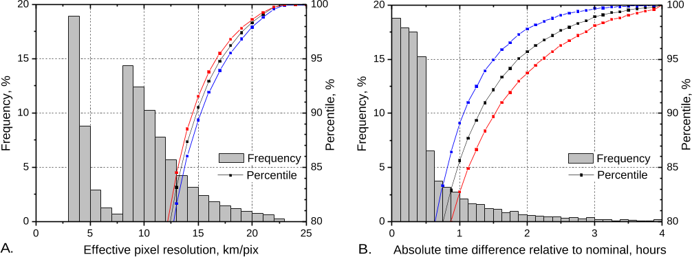
Figure 4. Frequency distribution of the effective pixel resolution (A) for characteristic time =5 hours. Overlaid on the same figure are percentiles of the effective pixel resolution calculated for =4 hours (blue curve), =5 hours (black), and =6 hours (red). Chart B shows distribution of the absolute time difference and its corresponding percentiles calculated for the same three cases of . 
Figure 9. A zoomed subset of the EPIC-view composite generated for reflectance in 0.63 m over the North Atlantic and North Africa for Sep-15-2015 13:23UTC (left) and the corresponding EPIC Level 1B data in band 0.68 m over the same area (right). 
Figure 5. A zoomed region of the composite brightness temperature reveals an uneven boundary between data from different satellites (A). The same region where cumulative probability distribution was used to mix the pixel data, which yields a smooth transition (B). 
Figure 6. Transition between two satellite ratings is made smoother by adding a random variable changing from –5% to +5%. The transition occurs between the two vertical grid lines. The solid curve below is the cumulative distribution function showing the probability that Sat2 rating is selected. 
Table 3. Summary of the satellite radiance, cloud property, and scene identification variables processed for EPIC-view composites: 
Figure 7. Conversion from a uniformly distributed random variable to a pseudo-normal distribution by using the tangent function. 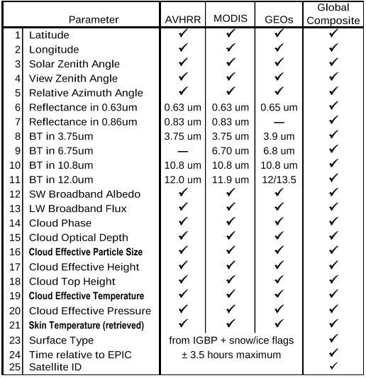
Table 1. List of parameters included in global composite. 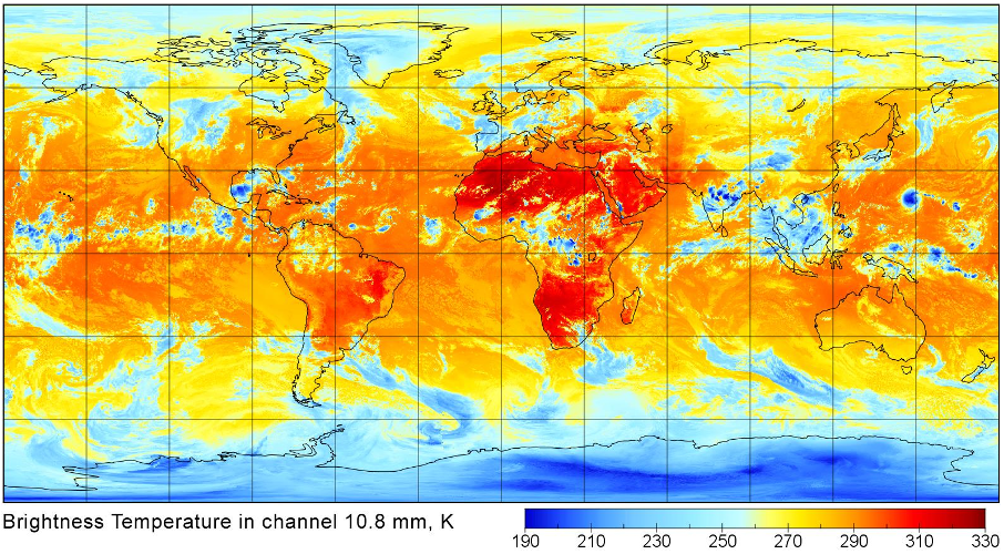
Figure 1. Global composite map of the brightness temperature in channel 10.8 m generated for Sep-15-2015 13:23UTC. The continuous coverage leaves no gaps and apparent disruptions in the temperature field. 
Table 2. Upper-left quarter of the matrix of PSF weights calculated for a half-pixel grid: 
Figure 8. Point spread functions of three adjacent pixels showing their overlapped fields of view. 
Figure 3. A map of the time relative to nominal for the case of Sep-15-2015 13:23UTC. Pale colors correspond to a lower difference in time and bright colors indicate a larger difference. 
Figure 2. A map of satellite coverage in a global composite generated for Sep-15-2015 13:23UTC.


02 Oct 2017-