
All figures (7)
 Figure 3. (a) Pacific and (b) Atlantic tide gauge cross-correlation at zero-lag. Each circular marker gives the the correlation rij , between gauge i and gauge j. Tide gauge are numbered in ascending order from south to north, following the coastline. Bolder circular contour indicates that the correlation is above significance level of 95%.
 Figure 1. (a) Kuroshio region circulation: The three Kuroshio paths — the typical Large Meander (tLM), the near-shore Non-Large Meander (nNLM) and the offshore Non-Large Meander (oNLM) are indicated upstream of the Izu-Ogasawara Ridge. The mean location of the KE is indicated offshore of this point showing the location of the quasi-stationary meanders. The Oyashio current is shown in blue. On land, K indicates Kyūshū, Hon stands for Honshū and Ho indicates Hokkaidō. (b) Gulf Stream region circulation from the Florida Current to the Gulf Stream Extension. The Northern Recirculation Gyre is also indicated. On land, M.-A. B. stands for Mid-Atlantic Bight and N.S. indicates Nova Scotia. Markers in (a) and (b) indicate the location of the tide gauges used in this study. The colour and shape of the markers in (a) and (b) indicate the angle used to rotate the wind stress in an alongshore/across-shore coordinate system for the removal of sea-level variability driven by local atmospheric effect (See Supplementary Table S1 and Supplementary Table S2). Shadings in (a) and (b) indicate bathymetry.
 Figure 2. (a) GS climatological position (solid line) and GS climatological position plus GSNW spatial amplitude based on EOF analysis of the along-jet temperature anomalies (dashed line). Conversion ratio from normalized temperature to latitude is arbitrarily set for visualisation, but is the same at every grid point. (c) GSNW time series obtained from EOF analysis (thick light blue), with also the GSNW index of Joyce et al. (2000) shown in red. (b) and (d) As for (a) and (c), but obtained for the Kuroshio Extension, and with the KE indices of Qiu et al. (2016) replacing Joyce et al. (2000). The solid orange line in (d) corresponds to the temperature and salinity based index, and the dashed thin red line corresponds to the wind-based index. All timeseries in (c) and (d) are normalized.
 Figure 5. (a) and (b) present the leading EOF (φ1) of the gridded, tide gauge obtained, sea-level anomaly (circular markers). (c) and (d) present, for the Pacific and Atlantic respectively, the associated principal components α1’s (solid blue lines), together with indices of extension meridional location: this study and Qiu et al. (2016) T/S-based and wind-based KEIs (on (c), thick light blue line, orange solid line and dot-dashed red line respectively); and this study and Joyce et al. (2000) GSNWs (on (d), thick light blue line and dot-dashed red line, respectively) . All quantities on (c) and (d) are normalized. Colour shadings on (a) and (b) are, for each basin, the sea surface velocity magnitude composites difference based on the principal component α1 (period of α1 >+2/3 minus period of α1 <−2/3). The arbitrary threshold of ±2/3 was used, but taking any number between zero and one leads to akin patterns. The inset on (a) present the regression coefficient obtained when the principal component is regressed on the original tide gauges, with a zoom in on the Kii peninsula.
 Figure 7. (a) Moving standard deviation of α2 with a 15 year running window (solid blue line) and moving correlation with the same windowing between the northern and southern Atlantic gauge grouping averages (red dashed line). The latter is the same as the blue line on Figure 4 (a). (b) Moving correlation with a 15 year running window between the second principal component α2 and our GSNW index (solid blue line), and between α2 and our GSNW index computed on 75°W – 69°W (dot-dashed red line).
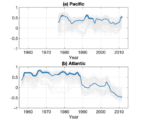 Figure 4. Moving correlation analysis between the tide gauges records with a running window of 15 years. Each individual grey line renders the moving correlation between two records. The x-axis represents the center of the moving window. (a) Cross correlation between the Oyashio and West of Kii groupings (grey lines). (b) Cross-correlation between gauges on either side of the Cape Hatteras, the separation point of the Gulf Stream (again, grey lines) On each panel, the solid blue line is the moving correlation between the group averages of sea-level anomalies. Significant correlations above 95% level are indicated by thicker blue line.
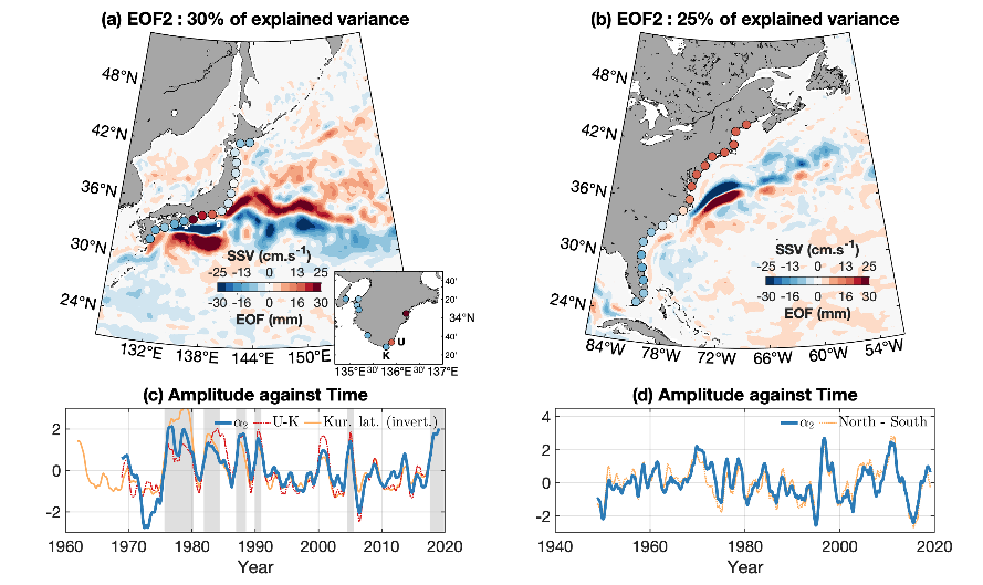 Figure 6. (a) and (b) present the second EOF (φ2) of the gridded, tide gauge obtained, sea-level anomaly (circular markers). (c) and (d) present, for the Pacific and Atlantic respectively, the associated principal components α2’s (solid blue lines). Also on (c), the Kuroshio southernmost latitude South of Tōkai is represented with the solid orange line (positive values indicate Kuroshio further to the south), the difference between sea level at Uragami and Kushimoto with the dot-dashed red line, and grey shadings represent periods of typical large meander (JMA, 2018). On (d), the dashed yellow line is the sea-level difference between the averages of northern and southern groupings of tide gauges, as in McCarthy et al. (2015). All timeseries on (c) and (d) are normalized. Colour shadings on (a) and (b) are, for each basin, the sea surface velocity magnitude composite difference based on the principal component α2 (period of α2 >+2/3 minus period of α2 <−2/3). The arbitrary threshold of ±2/3 was used, but taking any number between zero and one leads to akin patterns. The inset on (a) present the regression coefficient obtained when the principal component is regressed on the original tide gauges, with a zoom in on the Kii peninsula.


