
All figures (17)

Figure 4. Results of the 1-D inversions using VELEST. The 35 best (a) P wave and (b) S wave final velocity models (gray lines). Heat maps for the same (c) P wave and (d) S wave set of final models. The yellow lines indicate all initial velocity models used. The selected minimum 1-D models are indicated in black lines in panels (a) and (b), and in red lines in panels (c) and (d). 
Figure 10. Averaged DWS distribution at different depth levels. Panels (a) and (c) show two depth slices for the Vp model DWS distribution at −2.6 and −1.10 km depths. Panels (b) and (d) show the depth slices for the Vp/Vsmodel DWS distribution at −2.6 and −1.10 km depths. Darker shading indicates regions of higher ray density. 
Figure 14. Vpmodel variations with respect to the minimum 1-D velocity model at different depth levels. Panels (a)–(d) show depth slices for the resulting Vp model variations at −2.60, −2.10, −1.60, and −1.10 km depths, respectively. Green circles mark the location of earthquakes ±150m away from slice. Dashed red lines indicate the boundary at which spread values are less than or equal to 1.5. Gray areas mark the regions where the DWS is less than or equal to 5. 
Figure 5.Minimum 1-D model showing (a) the selected Vp and Vsmodels along with two available models (Lermo et al., 2008; Löer et al., 2020), (b) the resulting Vp/Vs ratio, and (c) the earthquake distribution over depth after the 1-D inversion. Solid lines indicate the depth intervals with best sensitivity for each model. 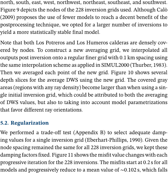
Figure 8. Cross Sections (a) A1-A1′ and (b) B1-B1′ for the Vpmodel DWS distribution (Figure 7). Darker shading indicates regions of higher ray density. Black crosses indicate the node positions. 
Figure 9. Nodes of the 228 inversion grids used to estimate the average velocities. 
Figure 13. Cross Sections A2-A2′ , B2-B2′ , C2-C2′ , and D2-D2′ (Figure 12) for the retrieved Vp and Vp/Vsmodel variations. Panels (a), (c), (e), and (g) show the recovered Vp anomalies, and panels (b), (d), (f), and (h) show the recovered Vp/Vs anomalies of the checkerboard test. Gray areas mark the regions where the DWS is less than or equal to 5. 
Figure 1. (a) Surface geology, (b) main structures, and well locations at LHVC (modified from Carrasco-Núñez, Hernández, et al., 2017; Norini et al., 2015). (c) Locations of the Trans-Mexican Volcanic Belt (TMVB) and LHVC (red triangle). 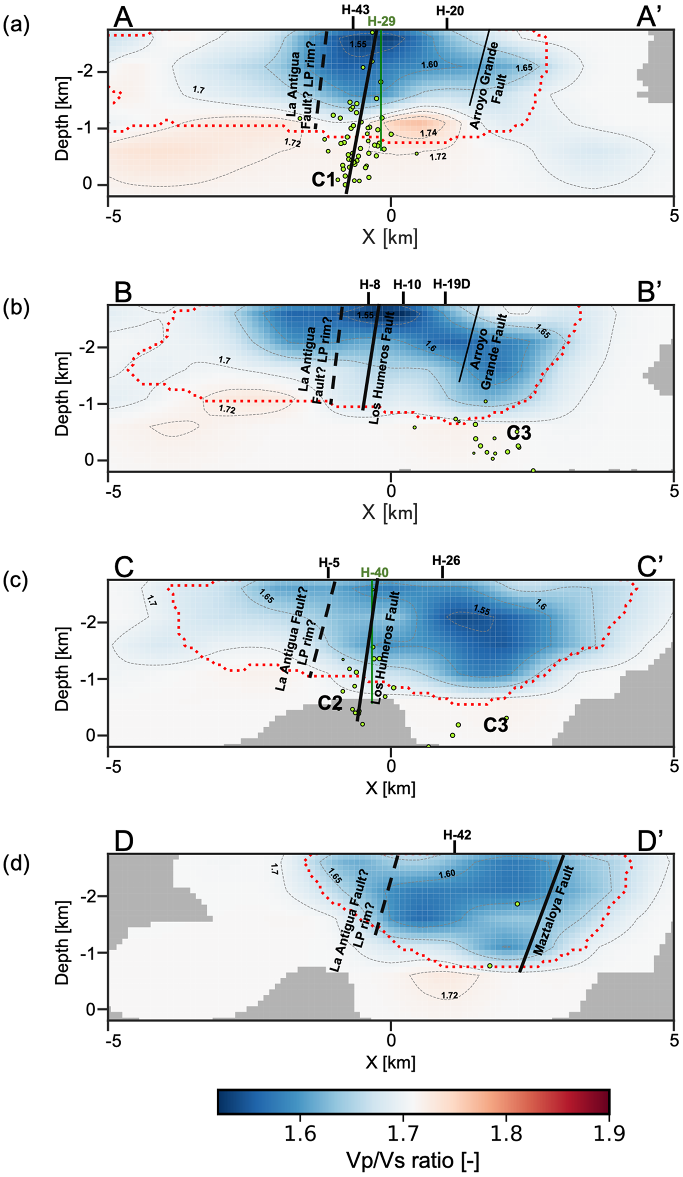
Figure 17. (a–d) Cross sections for the Vp/Vsmodel (Figure 16). Green circles mark the locations of earthquakes ±200m away from the slice. Dashed red lines indicate the boundary at which spread values are less than or equal to 1.5. Gray areas mark the regions where the DWS is less than or equal to 5. Approximate locations of main structures are indicated in black. Vertical green lines indicate the positions of neighboring injection wells. 
Figure 12. Checkerboard recovery. Panels (a), (c), and (e) show three depth slices for the recovered Vp anomalies at −2.6, −2.10, and −1.10 km depths. Panels (b), (d), and (f) show the recovered Vp/Vs anomalies at −2.6, −2.10, and −1.10 km depths. The red and blue squares mark the positions of the synthetic high- and low-velocity anomalies. Gray areas mark the regions where the DWS is less than or equal to 5. 
Figure 6. Raypath distribution after the 1-D inversion: (a) map view and (b) N-S and (c) E-W projections. Seismic stations are represented as purple triangles, and local events as green circles. The projections of three injection wells are marked as red lines in the cross sections. Dark solid lines in the map view indicate structures inferred at the surface, and the gray lines correspond to topographic contours. 
Figure 2. Topographic map and temporary seismic network at Los Humeros geothermal field. Blue and red triangles mark the positions of three component short-period (Mark L-4C-3D) and three-component broadband (Trillium Compact 120s) sensors, respectively. The reference station for the 1-D inversions (also a three-component broadband Trillium Compact 120s sensor) is marked as a red circle. Several identified and inferred structures are delineated in black (modified from Carrasco-Núñez, Hernández, et al., 2017; Norini et al., 2015). 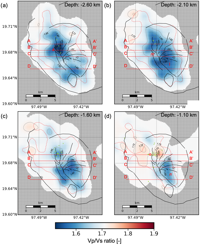
Figure 16. Vp /Vs structure at different depth levels. Panels (a)–(d) show depth slices for the resulting Vp/Vsmodel at −2.60, −2.10, −1.60, and −1.10 km depths, respectively. Green circles mark the locations of earthquakes ±150m away from the slice. Dashed red lines indicate the boundary at which spread values are less than or equal to 1.5. Gray areas mark the regions where the DWS is less than or equal to 5. 
Figure 11. RMS misfit variation for the 228 inverted models. 
Figure 7.Model parametrization and DWS distribution at different depth levels for an initial (unrotated) inversion grid. Panels (a) and (c) show two depth slices for the Vpmodel DWS distribution at −2.6 and −1.10 km depths. Panels (b) and (d) show the depth slices for the Vp/Vsmodel DWS distribution at −2.6 and −1.10 km depths. Darker shading indicates regions of higher ray density. Gray crosses indicate node positions. 
Figure 3. Distribution of the detected local earthquakes after a nonlinear localization in a homogeneous 3-D volume with a P wave velocity of 3.5 km/s and a Vp/Vs ratio of 1.73. Triangles mark the station positions, and dark solid lines indicate structures inferred at the surface. Red stars mark the positions of three injection wells. C1, C2, and C3 indicate the positions of three main seismic clusters. Depths are defined relative to sea level. 
Figure 15. (a–d) Cross sections for the Vpmodel variations (Figure 14). Green circles mark the locations of earthquakes ±200m away from the slice. Dashed red lines indicate the boundary at which spread values are less than or equal to 1.5. Gray areas mark the regions where the DWS is less than or equal to 5. Dashed gray lines indicate different absolute velocity levels, and solid gray lines mark approximate unit boundaries. Approximate locations of main structures are indicated in black. Vertical green lines indicate the positions of neighboring injection wells.


09 Mar 2020-