
All figures (13)
 Figure 6. Redshift distribution of galaxies in the NVSS–SDSS (top panel) and NVSS–SDSS–IRAS (middle panel) samples. The bottom panel shows the IR detection fraction as a function of redshift. Various galaxy types are indicated in the top right of the middle panel.
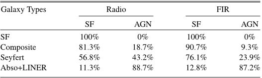 Table 2 Fractions of Star Formation and AGN Activity in Radio and FIR Regimes for Various Types of Galaxies
 Figure 12. FIR excess (Δ logLFIR) vs. radio excess (Δ logL1.4 GHz) for different types of NVSS–SDSS–IRAS galaxies (labeled in each panel) within a redshift range of 0.04–0.3. The FIR and radio excess has been defined as the difference in logarithm of the observed emission and that expected from their SFR, as given by the SED modeling (see Equation (5) and Figure 11 for details). Histograms on the axes show the distributions of the intrinsic Δ logL values. A Gaussian fit to the distribution of star-forming galaxies is also shown in each panel (solid line). In each panel, filled dots represent the galaxies, and the gray scale shows the distribution of star-forming galaxies to guide the eye. Lines of constant q are also shown.
 Figure 1. Distribution of distances between the radio and FIR detections for the NVSS-IRAS (full black line) and NVSS–SDSS–IRAS (dashed red line) samples. The cumulative distribution is shown in the inset.
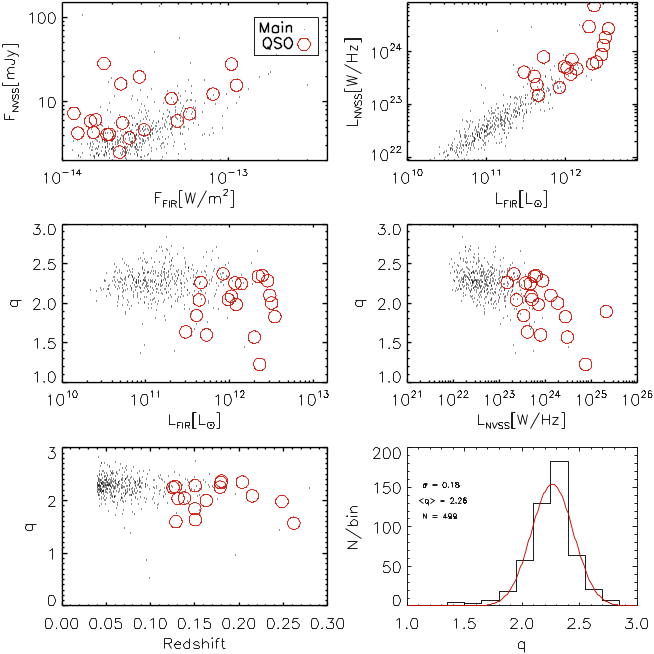 Figure 7. Radio–FIR correlation shown for the NVSS–SDSS–IRAS galaxies (dots) and quasars (open circles). The middle panels show the FIR/radio ratio (i.e., q parameter defined by Equation (1)) as a function of FIR (left) and radio (right) luminosities. Note a decrease in the q-value with increasing radio luminosity. The bottom panels show q as a function of redshift (left) and the distribution of q with its best-fit Gaussian (right). The number of objects in the sample (N), the biweighted mean FIR/radio ratio (〈q〉), and the dispersion (σ ) are indicated in the bottom right panel.
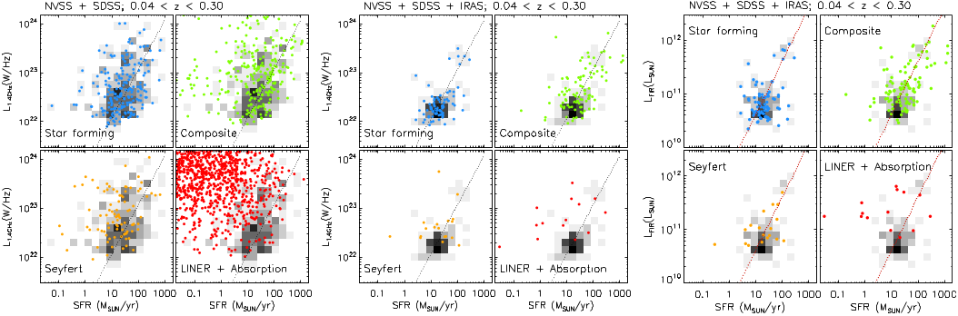 Figure 11. 1.4 GHz radio (left and middle panel) and FIR (right panel) luminosity as a function of SFR, derived via SED fitting to the NUV-NIR SDSS photometry (see the text for details). In the three large panels different galaxy types (symbols) and samples (indicated above and in each panel) are shown. The gray-scale histogram in each plot shows the distribution of star-forming galaxies for a given sample. Superimposed on the plots (dashed lines) are calibrations converting radio and FIR luminosity to SFR (Yun et al. 2001; Kennicutt 1998).
 Figure 10. FIR/radio ratio (q) as a function of redshift (left panel) and the distribution of q for 21 IR (IRAS) detected quasars (right panel) in our radio–IR–optical sample. Note that the median q-value for quasars is lower than the average q obtained for star-forming galaxies, but comparable to that obtained for Seyfert galaxies (see Figure 9). The source with q ∼ −1 is a strong radio source.
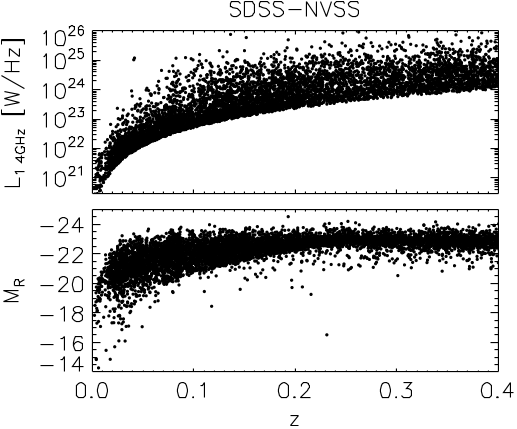 Figure 3. Top panel shows the 1.4 GHz luminosity as a function of redshift for the NVSS–SDSS galaxies. The bottom panel shows their absolute optical r-band magnitude (not K-corrected) as a function of redshift.
 Figure 2. Distribution of flux density at 20 cm (top panel) and 60 μm (bottom panel) for various radio-selected samples indicated in the top right of the panels. (A color version of this figure is available in the online journal.)
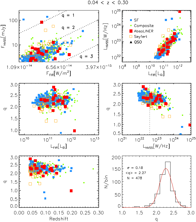 Figure 8. Equivalent to Figure 7, but for different galaxy types. The different symbols are indicated in the top right panel, and lines of constant q have been added to the top left panel.
 Figure 4. Top two panels are the same as Figure 3 but for NVSS–SDSS–IRAS galaxies. The bottom panel shows the FIR luminosity vs. redshift.
 Figure 9. Radio–FIR correlation shown for the NVSS–SDSS–IRAS galaxies divided (from top to bottom) into (a) absorption line galaxies, (b) LINERs, (c) Seyferts, (d) composite, and (e) star-forming galaxies. The left panels show the FIR–radio correlation slope, q, as a function of redshift. The right panels show the distribution of q for each class of galaxies in the redshift range 0.04 < z < 0.3, free of selection effects due to SDSS fiber sizes used for their optical spectroscopy.
 Figure 5. Optical spectroscopic diagnostic diagrams (see Kauffmann et al. 2003; Kewley et al. 2001, 2006) that separate emission-line galaxies into star-forming, composite galaxies, and various types of AGNs (Seyferts and LINERs). The top panel shows the SDSS–NVSS sample, and the bottom panel the SDSS–NVSS–IRAS galaxies. Large symbols represent unambiguously identified galaxies (see the text for details). Blue filled squares represent SF galaxies and green dots show composites. Red open squares and circles represent unambiguous Seyferts and LINERs, respectively.


