scispace - formally typeset
Open AccessJournal ArticleDOI

A Road Map for Efficiently Taxing Heterogeneous Agents

TLDR
The authors characterizes optimal labor income taxes that depend on age, household assets, and filing status (one or two earners) within a life-cycle model with heterogeneous, two-member households.
Abstract
This paper characterizes optimal labor income taxes that depend on age, household assets, and filing status (one or two earners) within a life-cycle model with heterogeneous, two-member households. The key innovation is a labor supply elasticity that varies endogenously among households. I find that tax distortions should be hump shaped in age, decrease in household assets, and be lower for joint relative to single filers. Age and assets act as complements within the optimal tax policy. Overall, a tax system using all three tags can increase consumption up to 6.4 percent and welfare up to 1.5 percent. (JEL D14, D91, H21, H24, J22, J31)

read more

Content maybe subject to copyright    Report

Online Appendix for “A Road Map for Efficiently Taxing
Heterogeneous Agents”
Marios Karabarbounis
Federal Reserve Bank of Richmond
August 5, 2015
A Alternative models: Aggregate Effects
This section reports the aggregate effects of the optimal labor-income policy in the “Ex-
ogenous Human Capital” model and the “Constant Elasticity Model.”
Table 1 reports the effects and welfare gains for the model with exogenous human capital.
Overall, the aggregate effects are in the same range. In addition, the presence of endogenous
human capital seems to add 0.1% to our welfare gains. Table 2 compares the effects of the
the age- and assets- dependent tax reform for both models. Changes in macro variables and
welfare gains are close to the ones found in the benchmark economy. Table 2 also reports the
effects in macro aggregates and welfare gains for different values of labor supply elasticity.
1
A larger value of labor supply elasticity can increase labor supply (and capital) by a larger
amount. However, welfare gains seem robust across specifications.
1
In the benchmark model the (heterogeneity in) labor supply elasticity depends mostly on the distribution
of reservation wages and not on the value θ (see Hansen (1985), Rogerson (1988), and Chang and Kim (2006)).
In contrast, varying parameter θ
c
in the CEM will affect uniformly all agents.
1

Table 1: Aggregate Effects of Tax Reform: Benchmark and Exogenous Human Capital
Model Benchmark Exogenous Human Capital
K +19.7% +20.3%
L +2.7% +2.8%
C +6.4% +6.0%
w +5.6% +5.7%
r -1.0% -1.0%
Cons. Gini -0.2% -0.5%
CEV +1.5% +1.4%
Note: The Table reports the percentage change in aggregates due to the tax reform. The tax reform includes age, household
assets, and filing status as tax tags. Results are presented for the benchmark case and two alternative specifications. A model
with exogenous human capital accumulation and a model with constant elasticity of labor supply.
Table 2: Aggregate Effects of Tax Reform: Benchmark and CEM
Model Benchmark CEM
θ
c
= 0.4 θ
c
= 0.73 θ
c
= 1.5
K +17.7% +18.9% +18.4% +22.2%
L +0.6% +0.6% +0.9% +1.7%
C +3.7% +3.0% +3.1% +4.2%
w +5.8% +6.1% +5.9% +6.8%
r -1.1% -0.3% -0.3% -0.4%
Cons. Gini +0.3% +0.2% +0.2% +0.2%
CEV +1.0% +1.1% +1.1% +1.0%
Note: The Table reports the percentage change in aggregates due to the tax reform. The tax reform includes age and household
assets as tax tags. Results are presented for the benchmark case and a model with constant elasticity of labor supply. For the
latter case, I present the effects of the optimal tax system for a variety of labor supply elasticities: θ
c
= 0.4,θ
c
= 0.73, θ
c
= 1.5.
B Simpler Policies
In this section, I restrict the age-dependent tax system to simpler forms. In particular, I
analyze a linear form, τ
00
+ τ
01
j, a second-degree polynomial, τ
00
+ τ
01
j + τ
02
j
2
, and compare
them to our benchmark specification: τ
00
+ τ
01
j + τ
02
j
2
+ τ
03
j
3
. The aggregate effects and
2

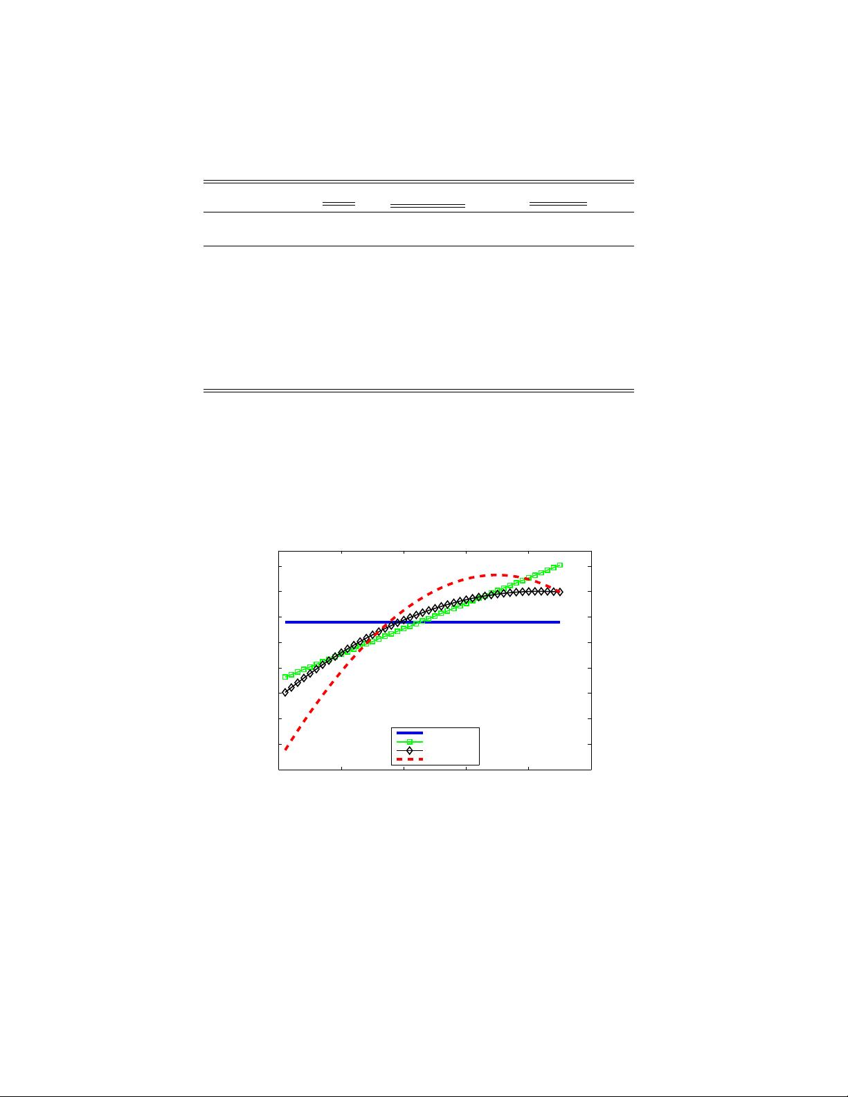
optimal tax properties are shown in Table 3 and Figure 1, respectively.
Table 3: Age-dependent Taxes: Simpler Functional Forms
Linear Second-Degree Benchmark
Functional Form τ
00
+ τ
01
j τ
00
+ τ
01
j + τ
02
j
2
τ
00
+ τ
01
j + τ
02
j
2
+ τ
03
j
3
K +5.3% +5.0% +9.5%
L -1.0% -0.7% +0.8%
C +0.1% +0.4% +0.9%
w +2.2% +2.0% +4.1%
r -0.4% -0.4% +0.6%
Cons. Gini -1.1% -1.3% -1.7%
CEV +0.2% +0.3% +0.4%
Note: The table reports the percentage change in aggregates due to an age-dependent tax reform. Results are presented for a
linear tax function, a second-degree polynomial and the benchmark specification.
Figure 1: Optimal Age-dependent Taxes: Simpler Functional Forms
20 30 40 50 60 70
−0.08
−0.03
0.02
0.07
0.12
0.17
0.22
0.27
0.32
τ
0
Age
Optimal Tax by Age
Current U.S.
Linear
Second Degree
Benchmark
Note: The figure plots the properties of optimal age-dependent taxes for different functional forms: linear, second-degree
polynomial and benchmark case (third-degree polynomial).
A linear increasing function increases capital by a smaller amount compared to the bench-
mark. Moreover, labor supply decreases as the tax distortion induces older households to
retire earlier. If the tax function is a second-degree polynomial then the tax distortion also
increases but a smaller rate for older households. This makes the employment reduction small-
3

er. Using the benchmark specification (third-degree polynomial), we can increase capital by a
larger amount but also increase employment. The flexibility allows to increase tax distortions
steeply up to age 50 and decrease taxes after that age. Although relatively small, welfare
gains double compared to a linear tax function.
C Household’s Problem: Value Functions
In this section, I write the value function for a household employing the female worker
V
{NE,E}
and a household whose members are not employed V
{NE,N E}
. The value function
for a household employing the female worker is:
V
{NE,E}
zj
(a, x, κ, E
1
) = max
c,a
0
,h
f
(
log(c) + ψ
m
j
(1 h
m
)
1θ
1 θ
+ ψ
f
j
(1 h
f
)
1θ
1 θ
ζ(E
f
1
)
+βs
j+1
X
x
m
0
X
x
f
0
Γ
x
m
x
0
m
Γ
x
f
x
0
f
[
(1 λ
m
)
1 p
X
s={2,3}
p
s
V
1
z(j+1)
(a
0
, x
0
, κ
s
, E) +
λ
m
1 p
X
s={2,3}
p
s
V
{NE,N E}
z(j+1)
(a
0
, x
0
, κ
s
, E)]
(1)
s.t. h
f
= 0 (2)
(1+τ
c
)c +a
0
= (1τ
ss
)W T
L
(W ; S)+(1+r(1τ
k
))(a +T r) (3)
E = {u, e} (4)
The value function for a household with no earners is:
4

V
{NE,N E}
zj
(a, x, κ, E
1
) = max
c,a
0
(
log(c) + ψ
m
j
(1 h
m
)
1θ
1 θ
+ ψ
f
j
(1 h
f
)
1θ
1 θ
+βs
j+1
X
x
m
0
X
x
f
0
Γ
x
m
x
0
m
Γ
x
f
x
0
f
V
2
z(j+1)
(a
0
, x
0
, κ
0
, E)]
(5)
s.t. h
m
= 0, h
f
= 0 (6)
(1+τ
c
)c+a
0
= (1+r(1τ
k
))(a+T r) (7)
E = {u, u} (8)
References
Chang, Y., and Kim, S.-B. (2006). “From individual to aggregate labor supply: a quantitative
analysis based on a heterogeneous agent macroeconomy”. International Economic Review,
47 (1), 1-27.
Hansen, G. D. (1985). “Indivisible labor and the business cycle”. Journal of Monetary
Economics, 16 (3), 309-327.
Rogerson, R. (1988). “Indivisible labor, lotteries and equilibrium”. Journal of Monetary
Economics, 21 (1), 3-16.
5
Citations
More filters
Book ChapterDOI

Macroeconomics and Household Heterogeneity

TL;DR: In this paper, the authors investigate how households in different segments of the wealth distribution were affected by income declines, and how they changed their expenditures differentially during the aggregate downturn and find that wealth inequality can significantly amplify the impact of an aggregate shock, and it does so if the distribution features a sufficiently large fraction of households with very little net worth that sharply increase their saving (i.e., they are not hand-to-mouth) as the recession hits.
Journal ArticleDOI

Health, health insurance, and retirement: a survey

TL;DR: The mechanisms through which health affects retirement are described and how these mechanisms interact with public pensions and public health insurance are discussed.
Journal ArticleDOI

The effects of collecting income taxes on Social Security benefits

TL;DR: In this paper, a detailed life-cycle model of labor supply, saving, and Social Security claiming is presented to assess the impact of Social Security benefits subject to income taxation, a provision that can significantly increase the marginal income tax rate for older individuals.
Journal ArticleDOI

Greater Inequality and Household Borrowing: New Evidence from Household Data

TL;DR: Coibion et al. as discussed by the authors show that low-income households in high-inequality regions (zip codes, counties, states) accumulated less debt relative to their income than low- income households in lower inequality regions.
Journal ArticleDOI

Effects of COVID-19 Early Release of Pension Funds. The Case of Chile

TL;DR: In this article, the authors quantified the effects of a 10% early release of pension funds and proposed four policies to mitigate these effects and address the current challenges of most defined contribution pension schemes.
References
More filters
Journal ArticleDOI

Self-insurance in a life-cycle model of labour supply and savings

TL;DR: In this article, the authors analyzed the incentives to work and to save over the life cycle in the presence of incomplete markets and found that flexibility in hours worked changes asset age-profiles: borrowing when young and saving when middle-aged are greater than when labour supply is fixed.
Journal ArticleDOI

Precautionary Savings or Working Longer Hours

TL;DR: In this paper, the authors quantified the macroeconomic implications of the lack of insurance against idiosyncratic labor market risk and showed that households make ample use of work effort as a consumption smoothing mechanism.
Journal ArticleDOI

Lifetime aggregate labor supply with endogenous workweek length

TL;DR: In this article, lifetime aggregate labor supply with endogenous workweek length was studied and it was shown that policies designed to increase the length of the working life may not increase aggregate lifetime labor supply.
Journal ArticleDOI

Social Security Reforms: Benefit Claiming, Labor Force Participation, and Long-Run Sustainability

TL;DR: In this paper, the authors assess the effects of these reforms on allocations and the solvency of the system in the long run and find that eligibility for Social Security and claiming of Social Security are not the same.
Journal ArticleDOI

Optimal Progressive Labor Income Taxation and Education Subsidies When Education Decisions and Intergenerational Transfers are Endogenous

TL;DR: The authors quantitatively characterize the optimal mix of progressive income taxes and education subsidies in a model with endogenous human capital formation, borrowing constraints, income risk and incomplete financial markets, and find that the welfare-maximizing fiscal policy is indeed characterized by a substantially progressive labor income tax code and a positive subsidy for college education.
Related Papers (5)
Frequently Asked Questions (4)
Q1. What are the contributions mentioned in the paper "Online appendix for “a road map for efficiently taxing heterogeneous agents”" ?

This section reports the aggregate effects of the optimal labor-income policy in the “ Exogenous Human Capital ” model and the “ Constant Elasticity Model. ” Table 1 reports the effects and welfare gains for the model with exogenous human capital. 

If the tax function is a second-degree polynomial then the tax distortion also increases but a smaller rate for older households. 

1In the benchmark model the (heterogeneity in) labor supply elasticity depends mostly on the distribution of reservation wages and not on the value θ (see Hansen (1985), Rogerson (1988), and Chang and Kim (2006)). 

The value function for a household employing the female worker is:V {NE,E} zj (a,x,κ,E−1) = maxc,a′,hf{ log(c) + ψmj (1− hm)1−θ1− θ + ψfj(1− hf )1−θ1− θ − ζ(Ef−1)+βsj+1 ∑ xm′ ∑ xf ′ Γxmx′mΓxfx′f ∗[ (1− λm) 1− p ∑s={2,3}psV 1z(j+1)(a ′,x′,κs,E) +λm 1− p ∑s={2,3}psV {NE,NE} z(j+1) (a ′,x′,κs,E)] (1)s.t. hf = 0 (2)(1+τc)c+a ′ = (1−τss)W −TL(W ; S)+(1+r(1−τk))(a+Tr) (3)E = {u, e} (4)The value function for a household with no earners is:V {NE,NE} zj (a,x,κ,E−1) = maxc,a′{ log(c) + ψmj (1− hm)1−θ1− θ + ψfj(1− hf )1−θ1− θ+βsj+1 ∑ xm′ ∑ xf ′ Γxmx′mΓxfx′f V 2 z(j+1)(a ′,x′,κ0,E)] (5)s.t. hm = 0, hf = 0 (6)(1+τc)c+a ′ = (1+r(1−τk))(a+Tr) (7)E = {u, u} (8)