scispace - formally typeset
Open AccessProceedings ArticleDOI

Cross-Field Joint Image Restoration via Scale Map

Reads0
Chats0
TLDR
A scale map is introduced as a competent representation to explicitly model derivative-level confidence and new functions and a numerical solver are proposed to effectively infer it following new structural observations.
Abstract
Color, infrared, and flash images captured in different fields can be employed to effectively eliminate noise and other visual artifacts. We propose a two-image restoration framework considering input images in different fields, for example, one noisy color image and one dark-flashed near infrared image. The major issue in such a framework is to handle structure divergence and find commonly usable edges and smooth transition for visually compelling image reconstruction. We introduce a scale map as a competent representation to explicitly model derivative-level confidence and propose new functions and a numerical solver to effectively infer it following new structural observations. Our method is general and shows a principled way for cross-field restoration.

read more

Content maybe subject to copyright    Report

Cross-Field Joint Image Restoration via Scale Map
Qiong Yan
§
Xiaoyong Shen
§
Li Xu
§
Shaojie Zhuo
Xiaopeng Zhang
Liang Shen
Jiaya Jia
§
§
The Chinese University of Hong Kong
Qualcomm Incorporated
http://www.cse.cuhk.edu.hk/leojia/projects/crossfield/
Abstract
Color, infrared, and flash images captured in different
fields can be employed to effectively eliminate noise and
other visual artifacts. We propose a two-image restoration
framework considerin g input images in different fields, for
example, one noisy color image and one dark-flashed near-
infrared image. The major issue in such a framework is
to handle structure divergence and find commonly usable
edges and smooth transition for visually compelling image
reconstruction. We introduce a scale map as a competent
representation to explicitly model derivative-level confi-
dence and propose new functions and a numerical solver
to effectively infer it following new structural observations.
Our method is general and shows a principled way for
cross-field restoration.
1. Introduction
Images captured in dim light are hardly satisfactory.
They could be very noisy when increasing ISO in a short
exposure duration. Using flash might improve lighting;
but it creates unwanted shadow and highlight, or changes
tone of the image. The methods of [6, 14, 1] restore a
color image based on flash and non-flash inputs of the same
scene. Recently, because of the popularity of other imaging
devices, more computational photography and computer
vision solutions based on images captured under different
configurations were developed.
For example, near infrared (NIR) images are with a sin-
gle channel recording infrared light reflected from objects
with spectrum ranging from 700nm-1000nm in wavelength.
NIR images contain many similar structures as visible co lor
ones when taken from the same camera position. This
enables a configuration to take an NIR image with less
noisy details by dark flash [11] to guide corresponding noisy
color image restoration. The main advantage is on only
using NIR flash invisible to naked human eyes, making
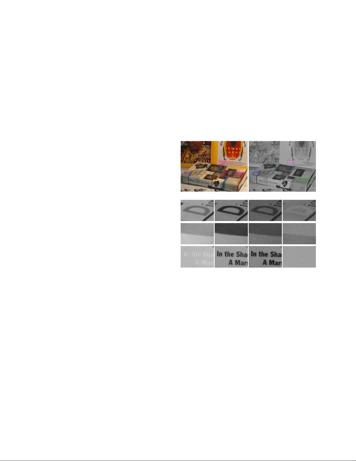
(a) RGB Image (b) NIR Image
(c) Close-up Comparison
Figure 1. Appearance comparison of RGB and NIR images. (a)
RGB image. (b) Corresponding NIR image. (c) Close-ups. The
four columns are for the R, G, B, and NIR channels respectively.
it a suitable way for daily portrait photography and of
remarkable practical importance.
In previous methods, Krishnan et al. [11] used gradients
of a dark-flashed image, capturing u ltraviolet (UV) and NIR
light to guide noise removal in the color image. Considering
rich details in NIR images, Zhang et al. [20] enhanced
the RGB counterpart by transferring contrast and details via
Haar wavelets. In [21] and [16], the detail layer was manip-
ulated differently for RGB and haze image enhancement.
Several methods also explore other image fusion appli-
cations in two-image deblurring [19], m atting [17], tone
mapping [7], upsampling [10], context enhancement [15],
relighting [2], to name a few. Bhat et al. [3] proposed
GradientShop to edit gradients, which can also be used to
enhance images.
1

We note existing methods work well for their respective
applications by handling different detail layers or gradients
from multip le images. But in terms of two-image high-
quality restoration, there remain a few major and fundamen-
tal issues that were not sufficiently addressed. We take the
RGB-NIR images shown in Fig. 1 as an example to reveal
the noticeable difference in detail distribution and intensity
formation. Structure inconsistency existing for many pixels
can be categorized as follows.
Gradient Magnitude Variation.Intherstrowof
Fig. 1(c), letter “D” is with different contrast. It is due
to varied reflectance to infrared and visible light.
Gradient Direction Divergence. In the second row,
edge gradients have opposite directions in the two
images, which cause structural deviation.
Gradient Loss. In the last row, the characters are
completely lost in the NIR image.
Shadow and Highlight by Flash. If one uses flash
only for the NIR image, it inevitably generates high-
light/shadow that is not contained in the other image.
Examples are presented later.
These issues are caused by inherent discrepancy of
structures in different types o f images, which we call cross-
field problems. The algorithms to address them can be
generally referred to as cross-field image restoration.Sim-
ple joint image filtering [18, 8] could blur weak edges due
to the inherent smoothing property. Directly transferring
guidance gradients to the noisy field also results in unnatural
appearance.
In this paper, we propose a framework via novel scale
map construction. This map captures the nature of structure
discrepancy between images and has clear statistical and
numerical meanings. Based on its analysis, we design
functions to form an optimal scale map considering adap-
tive smoothing, edge preservation, and guidance strength
manipulation. Aforementioned cross-field issues are dis-
cussed and addressed in this framework. We also develop
an effective solver via robust function approximation and
problem decomposition, which converges in less than 5
passes compared to other gradient decent alternatives that
may need tens or hundreds of iterations.
2. Modeling and Formulation
Our system takes the input of a noisy RGB image I
0
and a guidance image G captured from the same camera
position. G can be a dark-flashed NIR image or others
with possible structure variation as discussed above. Other
cross-field configurations are allowed in our framework,
presented in Section 4. Pixel values in each channel are
scaled to [0, 1]. G and I
0
could have different number of
channels. Our goal is to recover an image from I
0
with
Figure 2. Optimal scale map s computed from images in Fig. 1
according to Eq. (1). Dark to bright pixels correspond to negativ e
to positive values in different scales.
(a) 2D Images
(b) 1D Signal of Gradient
(c) 1D Signal of Maps
-0.2
-0.1
0
0.1
0.2
0.3
Gradient
-10
-5
0
5
10
s Map
Figure 3. 1D illustration. (a) Patch in the color image, NIR image
and s map. Plot (b) contains gradients along the vertical line in the
top two patches. (c) shows corresponding s values. Most of them
are zeros; positive and negative values also exist.
noise removed and structure retained. We process color
channels separately.
We introduce an auxiliary map s with the same size as
G, which is key to our method, to adapt structure of G to
that of I
the ground truth noise-free image. The s map is
defined under condition
min ∇I
s ·∇G. (1)
Here is an operator forming a vector with x-andy-
direction gradients. Each element s
i
in map s,where
i indexes pixels, is a scalar, measuring robust difference
between corresponding gradients in the two images. Simply
put, s is a ratio m a p between the guidance and latent images.
The optimal s corresponding to the cross-field example in
Fig. 1 is shown in Fig. 2, visualized as a color image after

pixel-wise value normalization to [0,1].
We analyze the properties of s with regard to structure
discrepancy between G and I
, and present them as
follows with the illustration in Fig. 3.
Property of s First, sign of each s
i
can be either positive
or negative. A negative s
i
means edges exist in the two
images, but with opposite directions, as demonstrated in
Fig. 3(c). Second, when the guidance image G contains
extra shadow and highlight caused by flash, which are
absent in I
, s
i
with value 0 can help ignore them.
Finally, s
i
can be any value when G
i
=0–thatis,
guidance edge does not exist, such as the red letters in Fig.
3(a). In this case, under local smoothness, s
i
being0isa
good choice.
In short, an optimal s map should be able to represent
all these structure discrepancies. It is first-of-a-kind to avail
cross-field restoration. Its additional benefit is the special
role as latent variables to develop an efficient optimization
procedure.
More of the Function We denote by I our estimate
towards I
. Eq. (1) is updated to
min ∇I s ·∇G. (2)
As it involves unknowns I and s, which correlate, the
functio n is ill-posed. We take its variation as a d ata term
expression, together with regularization on s, to construct
an objective function.
2.1. Data Term about s
In |s
i
G
i
−∇I
i
|,wherei indexes pixels, G
i
can be
analogously regarded as a scale map for s
i
due to the dual
relation between s
i
and G
i
. It controls the penalty when
computing s
i
for different pixels. The final cost resulted
from |s
i
G
i
−∇I
i
| is dependent on the value of G
i
.
For example, if G
i
and I
i
are doubled simultaneously,
although s remains the same, the cost from |s
i
G
i
−∇I
i
|
will get twice larger.
To stabilize costs w.r.t. s
i
, we perform normalization
i
|s
i
x
I
i
x
G
i
| + |s
i
y
I
i
y
G
i
|, (3)
which is modulated by the two components of G
i
.It
removes the unexpected scaling effect caused by G
i
.
Further to avoid the extreme situation when
x
G
i
or
y
G
i
is close to zero, and enlist the ability to r e ject outliers, we
define our data term as
E
1
(s, I)=
i
ρ(|s
i
p
i,x
x
I
i
|)+ρ(|s
i
p
i,y
y
I
i
|)
, (4)
where ρ is a robust function defined as
ρ(x)=|x|
α
, 0 <α<1. (5)
(a) Isotropic Smoothing (b) Anisotropic Smoothing
Figure 4. Isotropic versus anisotropic smoothing of the s map.
Result in (b) from anisotropic smoothing contains higher contrast
structure. The input images are shown in Fig. 5(a).
It is used to r emove estimation outliers. We set α =0.9
in experiments. p
i,k
,wherek ∈{x, y}, is a truncation
function
p
i,k
=
1
sign(
k
G
i
) · max(|∇
k
G
i
|)
, (6)
where sign(x) is the sign operator, outputting 1 if
k
G
i
is positive or zero and outputting -1 otherwise.
max(|∇
k
G
i
|) returns the larger value between |∇
k
G
i
|
and ε. The threshold ε is used to avoid division by zero and
is set to 0.004 empirically.
2.2. Data Term for I
ThedatatermforI is simply set as
E
2
(I)=
i
ρ(|I
i
I
0,i
|), (7)
where ρ is the same robust function and I
0,i
is the color
of pixel i in I
0
. E
2
(I) requires the restoration result not
to wildly deviate from the input noisy image I
0
especially
along salient edges. The robust function ρ helps reject part
of the noise from I
0
.
2.3. Regularization Term
Our regularization term is defined with anisotropic gra-
dient tensors [13, 4]. It is based on the fact that s values
are similar locally o nly in certain d irections. For instance, s
values should change smoothly or be constant along an edge
more than those across it. As shown in Fig. 4, uniformly
smoothing s in all directions blurs sharp edges.
Our anisotropic tensor scheme preserves sharp edges
according to gradient directions of G. By a few algebraic
operations, an anisotropic tenso r is expressed as
D(G
i
)=
1
(G
i
)
2
+2η
2
((G
i
)(G
i
)
T
+ η
2
1), (8)
where G
i
=(
y
G
i
, −∇
x
G
i
)
T
is a vector perpendicular
to G
i
, 1 is an identity matrix and scalar η controls the
isotropic smoothness. When G
i
is much smaller than

η, Eq. (8) degrades to 0.5 · 1 and the structure tensor is
therefore isotropic.
Generally, the two o rthogonal eigenvectors of D(G
i
)
are
v
i,1
=
G
i
|∇G
i
|
, v
i,2
=
G
i
|∇G
i
|
, (9)
with corresponding eigenvalues
μ
i,1
=
η
2
(G
i
)
2
+2η
2
i,2
=
(G
i
)
2
+ η
2
(G
i
)
2
+2η
2
. (10)
This decomposes the tensor to
D(G
i
)=
v
i,1
v
i,2
μ
i,1
0
0 μ
i,2

v
T
i,1
v
T
i,2
. (11)
This form makes it possible to express regularizatio n for
each s
i
as
E
3
(s
i
)=μ
i,1
(v
T
i,1
s
i
)
2
+ μ
i,2
(v
T
i,2
s
i
)
2
. (12)
Different smoothing penalties are contr olled by μ
i,1
and
μ
i,2
in directions v
i,1
and v
i,2
, across and along edges
respectively. Stronger smoothness is naturally imposed
along edges. The final smoothing term is thus defined as
E
3
(s)=
i
μ
i,1
(v
T
i,1
s
i
)
2
+ μ
i,2
(v
T
i,2
s
i
)
2
. (13)
2.4. Final Objective Function
The final objective function to estimate the s map and
restore image I is written as
E(s, I)=E
1
(s, I)+λE
2
(I)+βE
3
(s), (14)
where λ controls the confidence on noisy image I
0
,andβ
corresponds to smoothness of s. We describe their setting
in Section 4.
This objective function is non-convex due to the in-
volvement of sparsity terms. Joint representation for s and
I in optimization f urther complicates it. Naive gradient
decent cannot guarantee optimality and leads to very slow
convergence even for a local minimum. We contrarily
propose an iterative method, which finds constraints to
shape the s map according to its characteristics and yields
the effect to remove intensive noise from input I
0
.
3. Numerical Solution
To solve the non-convex function E(s, I) defined in
Eq. (14), we employ the iterative reweighted least squares
(IRLS), which make it possible to convert the original
problem to a few corresponding linear systems without
losing generality. This process, however, is still nontrivial
and needs a few derivations.
Initially, robust function ρ(x) in Eq. (5) for any scalar x
can be written as x
2
/|x|
2α
, further approximated as
ρ(x) φ(x) · x
2
, (15)
where φ(x) is defined as
φ(x)=
1
|x|
2α
+
. (16)
is a small number to avoid division by 0. We set it to
1E 4 empirically. This form splits the robust function into
two parts where φ(x) can be regarded as a weight for x
2
.In
our method, following the tradition of IRLS, φ(x) and x
2
are updated alternatively during optimization because each
of them can work together with other n ecessary terms to
form simpler representations, profiting optimization.
Vector Form To ease derivation, we re -write Eq. (14) in
the vector form by taking the expression in Eq. (15) into
computation. It yields
E(s, I)=(s P
x
C
x
I)
T
A
x
(s P
x
C
x
I)
+(s P
y
C
y
I)
T
A
y
(s P
y
C
y
I)
+ λ(I I
0
)
T
B(I I
0
)+βs
T
Ls, (17)
where s, I,andI
0
are vector representations of s, I,and
I
0
. C
x
and C
y
are discrete backward difference matrices
that are used to compute image gradients in the x and
ydirections. P
x
, P
y
, A
x
, A
y
and B are diagonal matrices,
whose i-th diagonal elements are defined as
(P
x
)
ii
= p
i,x
, (A
x
)
ii
= φ(s
i
p
i,x
x
I
i
),
(P
y
)
ii
= p
i,y
, (A
y
)
ii
= φ(s
i
p
i,y
y
I
i
),
B
ii
= φ(I
i
I
0,i
).
Among them, A
x
, A
y
and B account for the re-weighting
process and are typically computed using estimates from
prev ious iterations P
x
and P
y
are normalization terms
from the guidance image. The first three terms in Eq. (17)
correspond to terms E
1
and E
2
; s
T
Ls is created by E
3
.
Note the last term s
T
Ls controls spatial smoothness of s,
where matrix L is a smoothing Laplacian, expressed as
L = C
T
x
1
V
2
x
2
V
2
y
)C
x
+ C
T
y
2
V
2
x
1
V
2
y
)C
y
+2C
T
y
1
Σ
2
)V
x
V
y
C
x
(18)
after a bit complicated derivations. Σ
1
, Σ
2
, V
x
,andV
y
are
all d iagonal matrices. Their i-th diagonal elements are
1
)
ii
= μ
i,1
, (V
x
)
ii
=
x
G
i
/ max(|∇G
i
|),
2
)
ii
= μ
i,2
, (V
y
)
ii
=
y
G
i
/ max(|∇G
i
|).

Algorithm 1 Cross-Field Image Restoration.
1: input: noisy image I
0
, guidance image G, parameters
β and λ
2: initialize I I
0
, s 1
3: repeat
4: estimate s according to Eq. (21)
5: estimate I according to Eq. (23)
6: until convergence
7: output: s map and restored image I
Analysis We note L is actually an inhomogeneous term,
reflecting the anisotropic property of our smoothing regu-
larizer. To understand it, consider the extreme case that G
approaches zero. It leads to Σ
1
2
and V
x
= V
y
=
0,makingL a homogenous Laplacian. The resulting s
map is therefore smooth in all directions. But in natural
images, G on an edge is not isotropic and should be with
nonuniform regularization strength. Also, sparse C
x
and
C
y
lead to the sparse Laplacian matrix L, which facilitates
optimization b ecause many mature sparse-matrix solvers
exist in this community already.
3.1. Solver
We solve f or s and I based on above derivations. Results
of s and I in each iteration t are denoted as s
(t)
and I
(t)
.
Initially, we set s
(0)
= 1, whose elements are all 1sand
I
(0)
= I
0
.
By setting all initial s
i
to 1s, total smoothness is ob-
tained. It yields zero cost for E
3
(s), a nice starting point
for optimization. This initialization also makes the starting
I same as G with many details. Then at iteration t +1,
we solve two subproblems alternatively
Given s
(t)
and I
(t)
, minimize E(s, I
(t)
) to get s
(t+1)
.
Given s
(t+1)
and I
(t)
, minimize E(s
(t+1)
, I) to update
I
(t+1)
.
The procedure is repeated until s and I do not change
too much. Usually, 4-6 iterations are enough to generate
visually compelling results. The algorithm is depicted in
Algorithm 1, with the solvers elaborated on as follows.
Solve for s
(t+1)
The energy function with respect to s can
be expressed as
E(s)=(s P
x
C
x
I)
T
A
x
(s P
x
C
x
I)
+(s P
y
C
y
I)
T
A
y
(s P
y
C
y
I)+βs
T
Ls. (19)
Computation of A
x
and A
y
depends on estimates s and I
from the previous iteration. We denote by A
t,t
x
and A
t,t
y
the
matrices computed with s
(t)
and I
(t)
, which lead to
˜
E(s)=(s P
x
C
x
I
(t)
)
T
A
t,t
x
(s P
x
C
x
I
(t)
)
+(s P
y
C
y
I
(t)
)
T
A
t,t
y
(s P
y
C
y
I
(t)
)+βs
T
Ls.
(20)
It is simply quad ratic. Taking derivatives on s and setting
them to 0s, we obtain the sparse linear system
(A
t,t
x
+A
t,t
y
+βL)s = A
t,t
x
P
x
C
x
I
(t)
+A
t,t
y
P
y
C
y
I
(t)
. (21)
We solved it using pre-conditioned conjugate gradient
(PCG). The solution is denoted as s
(t+1)
.
Solve for I
(t+1)
Similarly, the energy function to solve for
I is given by
˜
E(I)=(s
(t+1)
P
x
C
x
I)
T
A
t+1,t
x
(s
(t+1)
P
x
C
x
I)
+(s
(t+1)
P
y
C
y
I)
T
A
t+1,t
y
(s
(t+1)
P
y
C
y
I)
+ λ(I I
0
)
T
B
t+1,t
(I I
0
), (22)
where A
t+1,t
x
and A
t+1,t
y
are calcu lated with available s
(t+1)
and I
(t)
. B
t+1,t
depends on I
(t)
. The final linear system in
the matrix form is
(C
T
x
(P
x
)
2
A
t+1,t
x
C
x
+ C
T
y
(P
y
)
2
A
t+1,t
y
C
y
)+λB
t+1,t
I
=(C
T
x
P
x
A
t+1,t
x
+ C
T
y
P
y
A
t+1,t
y
)s + λB
t+1,t
I
0
. (23)
The linear system is also solved using PCG and the solution
is denoted as I
(t+1)
.
3.2. Why Does It Work?
According to the linear system defined in Eq. (21), the
resulting s
i
for pixel i is a weighted average of p
i,x
x
I
i
x
I
i
/
x
G
i
and p
i,y
y
I
i
≈∇
y
I
i
/
y
G
i
, whose weights
are determined by (A
x
)
ii
and (A
y
)
ii
. Even if these weights
are quite different due to noise or other aforementioned
issues described in Section 1, our method can still get a
reasonable solution. We explain why this happens.
Assuming p
i,x
x
I
i
is larger than the other term, in
solving for I according to Eq. (23), s
i
reduces the gradient
in the x-direction and increases the other so that I
i
lies
close to sG
i
. In the meantime, noise is reduced. Then
after each iteration, a less noisy I is p ut into Eq. (21) to
produce new p
i,x
x
I
i
and p
i,x
y
I
i
, which are closer than
those in previous iterations.
Eventually when the two estimates meet each other, s
converges; I is accordingly optimal. The smoothness term
L in Eq. (21) helps avoid discontinuity in the s map along
edges of G .
We show in Fig. 5(e) the initial constant s map. (f)-
(g) are maps produced in two iterations, and (h) shows the
final s. Initially the map is noisy because of confusing
or contradictive gradient magnitudes and directions in the

Citations
More filters
Journal ArticleDOI

Adaptive Quantile Sparse Image (AQuaSI) Prior for Inverse Imaging Problems

TL;DR: The Adaptive Quantile Sparse Image (AQuaSI) prior as mentioned in this paper is based on a quantile filter, which can be used as a joint filter on guidance data, and can be readily plugged into a wide range of numerical optimization algorithms.
Journal ArticleDOI

Interpretable Multi-Modal Image Registration Network Based on Disentangled Convolutional Sparse Coding

TL;DR: Zhang et al. as discussed by the authors propose an interpretable multi-modal image registration network (InMIR-Net), which disentangles the multi-mode features that are responsible for alignment (RA features) from those that are not responsible for aligning (nRA features).
Journal ArticleDOI

Exploiting Non-Local Priors via Self-Convolution for Highly-Efficient Image Restoration

TL;DR: Guo et al. as discussed by the authors proposed a self-convolution operator to exploit image non-local properties in a unified framework, which can generalize the commonly-used nonlocal modeling methods, as well as produce results equivalent to standard methods.
Journal ArticleDOI

Scale-Aware Multispectral Fusion of RGB and NIR Images Based on Alternating Guidance

TL;DR: Experimental results show that the proposed scale-aware multispectral fusion of RGB and NIR images based on alternating guidance achieves good performance in noise reduction, detail transfer and color reproduction, and is superior to the state-of-the-art ones in terms of quantitative measurement and computational efficiency.
Journal ArticleDOI

Sensitivity Improvement of Extremely Low Light Scenes with RGB-NIR Multispectral Filter Array Sensor.

TL;DR: The results show that the proposed color restored image post-processing method to improve the sensitivity and resolution of an RGB-NIR MFA is effective, while maintaining the NIR pixel resolution characteristics, and improving the sensitivity in terms of the signal-to-noise ratio by approximately 13 dB.
References
More filters
Journal ArticleDOI

Scale-space and edge detection using anisotropic diffusion

TL;DR: A new definition of scale-space is suggested, and a class of algorithms used to realize a diffusion process is introduced, chosen to vary spatially in such a way as to encourage intra Region smoothing rather than interregion smoothing.
Proceedings ArticleDOI

Bilateral filtering for gray and color images

TL;DR: In contrast with filters that operate on the three bands of a color image separately, a bilateral filter can enforce the perceptual metric underlying the CIE-Lab color space, and smooth colors and preserve edges in a way that is tuned to human perception.
Journal ArticleDOI

Image Denoising by Sparse 3-D Transform-Domain Collaborative Filtering

TL;DR: An algorithm based on an enhanced sparse representation in transform domain based on a specially developed collaborative Wiener filtering achieves state-of-the-art denoising performance in terms of both peak signal-to-noise ratio and subjective visual quality.
Journal ArticleDOI

Single Image Haze Removal Using Dark Channel Prior

TL;DR: A simple but effective image prior - dark channel prior to remove haze from a single input image is proposed, based on a key observation - most local patches in haze-free outdoor images contain some pixels which have very low intensities in at least one color channel.
Book ChapterDOI

Guided image filtering

TL;DR: The guided filter is demonstrated that it is both effective and efficient in a great variety of computer vision and computer graphics applications including noise reduction, detail smoothing/enhancement, HDR compression, image matting/feathering, haze removal, and joint upsampling.
Related Papers (5)
Frequently Asked Questions (13)
Q1. What are the three common IRLS terms?

Among them, Ax, Ay and B account for the re-weighting process and are typically computed using estimates from previous iterations – Px and Py are normalization terms from the guidance image. 

because of the popularity of other imaging devices, more computational photography and computer vision solutions based on images captured under different configurations were developed. 

To solve the non-convex function E(s, I) defined in Eq. (14), the authors employ the iterative reweighted least squares (IRLS), which make it possible to convert the original problem to a few corresponding linear systems without losing generality. 

The authors contrarily propose an iterative method, which finds constraints to shape the s map according to its characteristics and yields the effect to remove intensive noise from input I0. 

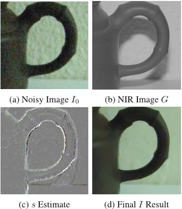
The restoration result shown in (d) is with much less highlight and shadow, which is impossible to achieve by gradient transfer or joint filtering. 

Their estimated s map shown in (c) contains large values along object boundaries, and has close-to-zero values for highlight and shadow. 

Since the two input images are color ones under visible light, the authors use each channel from the flash image to guide image restoration in the corresponding channel of the nonflash noisy image. 

The authors introduce an auxiliary map s with the same size as G, which is key to their method, to adapt structure of G to that of I∗ – the ground truth noise-free image. 

The limitation of their current method is on the situation that the guidance does not exist, corresponding to zero∇G and non-zero ∇I∗ pixels. 

This enables a configuration to take an NIR image with less noisy details by dark flash [11] to guide corresponding noisy color image restoration. 

Further to avoid the extreme situation when∇xGi or∇yGi is close to zero, and enlist the ability to reject outliers, the authors define their data term asE1(s, I) = ∑i( ρ(|si −pi,x∇xIi|)+ρ(|si−pi,y∇yIi|) ) , (4)where ρ is a robust function defined asρ(x) = |x|α, 0 < α < 1. (5)It is used to remove estimation outliers. 

In previous methods, Krishnan et al. [11] used gradients of a dark-flashed image, capturing ultraviolet (UV) and NIR light to guide noise removal in the color image. 

The final linear system in the matrix form is((CTx (Px) 2At+1,tx Cx + C T y (Py) 2At+1,ty Cy) + λB t+1,t ) I= (CTx PxA t+1,t x + C T y PyA t+1,t y )s + λBt+1,tI0. (23)The linear system is also solved using PCG and the solution is denoted as I(t+1).