scispace - formally typeset
Open AccessJournal ArticleDOI

Bayesian Estimation Supersedes the t Test

John K. Kruschke
- 01 May 2013 - 
- Vol. 142, Iss: 2, pp 573-603
Reads0
Chats0
TLDR
Bayesian estimation for 2 groups provides complete distributions of credible values for the effect size, group means and their difference, standard deviations and their Difference, and the normality of the data.
Abstract
Bayesian estimation for 2 groups provides complete distributions of credible values for the effect size, group means and their difference, standard deviations and their difference, and the normality of the data. The method handles outliers. The decision rule can accept the null value (unlike traditional t tests) when certainty in the estimate is high (unlike Bayesian model comparison using Bayes factors). The method also yields precise estimates of statistical power for various research goals. The software and programs are free and run on Macintosh, Windows, and Linux platforms.

read more

Content maybe subject to copyright    Report

Bayesian Estimation Supersedes the t-Test
Mike Meredith and John Kruschke
October 13, 2021
1 Introduction
The BEST package provides a Bayesian alternative to a t test, providing much richer information
about the samples and the difference in means than a simple p value.
Bayesian estimation for two groups provides complete distributions of credible values for the
effect size, group means and their difference, standard deviations and their difference, and the
normality of the data. For a single group, distributions for the mean, standard deviation and
normality are provided. The method handles outliers.
The decision rule can accept the null value (unlike traditional t tests) when certainty in the
estimate is high (unlike Bayesian model comparison using Bayes factors).
The package also provides methods to estimate statistical power for various research goals.
2 The Model
To accommodate outliers we describe the data with a distribution that has fatter tails than the
normal distribution, namely the t distribution. (Note that we are using this as a convenient
description of the data, not as a sampling distribution from which p values are derived.) The
relative height of the tails of the t distribution is governed by the shape parameter ν: when ν
is small, the distribution has heavy tails, and when it is large (e.g., 100), it is nearly normal.
Here we refer to ν as the normality parameter.
The data (y) are assumed to be independent and identically distributed (i.i.d.) draws from
a t distribution with different mean (µ) and standard deviation (σ) for each population, and
with a common normality parameter (ν), as indicated in the lower portion of Figure 1.
The default priors, with priors = NULL, are minimally informative: normal priors with
large standard deviation for (µ), broad uniform priors for (σ), and a shifted-exponential prior
for (ν), as described by Kruschke (2013). You can specify your own priors by providing a
list: population means (µ) have separate normal priors, with mean muM and standard deviation
muSD; population standard deviations (σ) have separate gamma priors, with mode sigmaMode
and standard deviation sigmaSD; the normality parameter (ν) has a gamma prior with mean
nuMean and standard deviation nuSD. These priors are indicated in the upper portion of Figure 1.
For a general discussion see chapters 11 and 12 of Kruschke (2015).
1

Figure 1: Hierarchical diagram of the descriptive model for robust Bayesian estimation.
3 Preparing to run BEST
BEST uses the JAGS package (Plummer, 2003) to produce samples from the posterior distribu-
tion of each parameter of interest. You will need to download JAGS from http://sourceforge.
net/projects/mcmc-jags/ and install it before running BEST.
BEST also requires the packages rjags and coda, which should normally be installed at the
same time as package BEST if you use the install.packages function in R.
Once installed, we need to load the BEST package at the start of each R session, which will
also load rjags and coda and link to JAGS:
> library(BEST)
4 An example with two groups
4.1 Some example data
We will use hypothetical data for reaction times for two groups (N
1
= N
2
= 6), Group 1
consumes a drug which may increase reaction times while Group 2 is a control group that
consumes a placebo.
> y1 <- c(5.77, 5.33, 4.59, 4.33, 3.66, 4.48)
> y2 <- c(3.88, 3.55, 3.29, 2.59, 2.33, 3.59)
Based on previous experience with these sort of trials, we expect reaction times to be approxi-
mately 6 secs, but they vary a lot, so we’ll set muM = 6 and muSD = 2. We’ll use the default priors
for the other parameters: sigmaMode = sd(y), sigmaSD = sd(y)*5, nuMean = 30, nuSD = 30),
where y = c(y1, y2).
> priors <- list(muM = 6, muSD = 2)
2

4.2 Running the model
We run BESTmcmc and save the result in BESTout. We do not use parallel processing here,
but if your machine has at least 4 cores, parallel processing cuts the time by 50%.
> BESTout <- BESTmcmc(y1, y2, priors=priors, parallel=FALSE)
Compiling model graph
Resolving undeclared variables
Allocating nodes
Graph information:
Observed stochastic nodes: 12
Unobserved stochastic nodes: 5
Total graph size: 51
Initializing model
|++++++++++++++++++++++++++++++++++++++++++++++++++| 100%
Sampling from the posterior distributions:
|**************************************************| 100%
4.3 Basic inferences
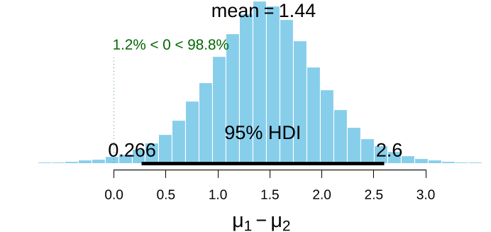
The default plot (Figure 2) is a histogram of the posterior distribution of the difference in
means.
> plot(BESTout)
Difference of Means
µ
1
µ
2
0.0 0.5 1.0 1.5 2.0 2.5 3.0
95% HDI
0.266 2.6
mean = 1.44
1.2% < 0 < 98.8%
Figure 2: Default plot: posterior probability of the difference in means.
Also shown is the mean of the posterior probability, which is an appropriate point estimate
of the true difference in means, the 95% Highest Density Interval (HDI), and the posterior
probability that the difference is greater than zero. The 95% HDI does not include zero, and
3

Difference of Means
µ
1
µ
2
0.0 0.5 1.0 1.5 2.0 2.5 3.0
95% HDI
0.266 2.6
mean = 1.44
19.9% < 1 < 80.1%
1% in ROPE
Figure 3: Posterior probability of the difference in means with compVal=1.0 and ROPE ± 0.1.
the probability that the true value is greater than zero is shown as 98.8%. Compare this with
the output from a t test:
> t.test(y1, y2)
Welch Two Sample t-test
data: y1 and y2
t = 3.7624, df = 9.6093, p-value = 0.003977
alternative hypothesis: true difference in means is not equal to 0
95 percent confidence interval:
0.6020466 2.3746201
sample estimates:
mean of x mean of y
4.693333 3.205000
Because we are dealing with a Bayesian posterior probability distribution, we can extract
much more information:
We can estimate the probability that the true difference in means is above (or below) an
arbitrary comparison value. For example, an increase reaction time of 1 unit may indicate
that users of the drug should not drive or operate equipment.
The probability that the difference in reaction times is precisely zero is zero. More inter-
esting is the probability that the difference may be too small to matter. We can define a
region of practical equivalence (ROPE) around zero, and obtain the probability that the
true value lies therein. For the reaction time example, a difference of ± 0.1 may be too
small to matter.
> plot(BESTout, compVal=1, ROPE=c(-0.1,0.1))
The annotations in (Figure 3) show a high probability that the reaction time increase is > 1.
In this case it’s clear that the effect is large, but if most of the probability mass (say, 95%) lay
within the ROPE, we would accept the null value for practical purposes.
4

Difference of Std. Dev.s
σ
1
σ
2
−2 −1 0 1 2
95% HDI
−1.08 1.41
mode = 0.1
36.4% < 0 < 63.6%
Figure 4: Posterior plots for difference in standard deviation.
BEST deals appropriately with differences in standard deviations between the samples and
departures from normality due to outliers. We can check the difference in standard deviations
or the normality parameter with plot (Figure 4).
> plot(BESTout, which="sd")
The summary method gives us more information on the parameters of interest, including
derived parameters:
> summary(BESTout)
mean median mode HDI% HDIlo HDIup compVal %>compVal
mu1 4.750 4.735 4.715 95 3.880 5.66
mu2 3.310 3.290 3.266 95 2.592 4.09
muDiff 1.440 1.442 1.435 95 0.266 2.60 0 98.8
sigma1 1.000 0.886 0.736 95 0.379 1.92
sigma2 0.829 0.731 0.615 95 0.313 1.61
sigmaDiff 0.170 0.143 0.100 95 -1.084 1.41 0 63.6
nu 34.927 25.751 9.796 95 0.849 96.97
log10nu 1.375 1.411 1.540 95 0.550 2.11
effSz 1.680 1.658 1.612 95 0.190 3.24 0 98.8
Here we have summaries of posterior distributions for the derived parameters: difference
in means (muDiff), difference in standard deviations (sigmaDiff) and effect size (effSz). As
with the plot command, we can set values for compVal and ROPE for each of the parameters of
interest:
> summary(BESTout, credMass=0.8, ROPEm=c(-0.1,0.1), ROPEsd=c(-0.15,0.15),
compValeff=1)
mean median mode HDI% HDIlo HDIup compVal %>compVal ROPElow
mu1 4.750 4.735 4.715 80 4.216 5.235
5

Citations
More filters
Journal ArticleDOI

Using Bayes to get the most out of non-significant results

TL;DR: It is argued Bayes factors allow theory to be linked to data in a way that overcomes the weaknesses of the other approaches, and provides a coherent approach to determining whether non-significant results support a null hypothesis over a theory, or whether the data are just insensitive.
Book

Doing Bayesian Data Analysis: A Tutorial with R, JAGS, and Stan

TL;DR: Doing Bayesian Data Analysis: A Tutorial with R, JAGS, and Stan provides an accessible approach to Bayesian data analysis, as material is explained clearly with concrete examples.
Journal ArticleDOI

Extensive impact of non-antibiotic drugs on human gut bacteria

TL;DR: For example, this paper screened more than 1,000 marketed drugs against 40 representative gut bacterial strains, and found that 24% of the drugs with human targets, including members of all therapeutic classes, inhibited the growth of at least one strain in vitro.
Journal ArticleDOI

Is psychology suffering from a replication crisis? What does "failure to replicate" really mean?

TL;DR: This article suggests that so-called failures to replicate may not be failures at all, but rather are the result of low statistical power in single replication studies, and of failure to appreciate the need for multiple replications in order to have enough power to identify true effects.
Journal ArticleDOI

The Bayesian New Statistics: Hypothesis testing, estimation, meta-analysis, and power analysis from a Bayesian perspective

TL;DR: In this paper, the authors compare Bayesian and frequentist approaches to hypothesis testing and estimation with confidence or credible intervals, and explain how Bayesian methods achieve the goals of the New Statistics better than frequentist methods.
References
More filters
Journal ArticleDOI

Stopping rules for clinical trials incorporating clinical opinion

TL;DR: A method is described of eliciting a range of differences between two treatments over which a group of clinical trial participants would have no clear preference for either treatment using an extension of the group sequential design.
Journal ArticleDOI

Inference by Eye: Pictures of Confidence Intervals and Thinking About Levels of Confidence

TL;DR: In this article, the authors discuss pictures taken from interactive software that suggest several ways to think about the level of confidence of a CI, p-values, and what conclusions can be drawn from inspecting a CI.
Journal ArticleDOI

Practical Bayesian design and analysis for drug and device clinical trials.

TL;DR: This paper provides illustrations in two applied settings where incorporation of available historical information is crucial, one concerning an AIDS drug trial and the other a comparison of left ventricular assist devices (LVADs), especially as implemented in the popular BUGS software package.
Journal ArticleDOI

Bayesian Inference and Application of Robust Growth Curve Models Using Student's t Distribution

TL;DR: In this article, the robust latent basis growth curve model is proposed to model the mathematical growth trajectory of mathematical development data and reveal the individual differences in mathematical development by using data augmentation and Gibbs sampling algorithms.
Frequently Asked Questions (8)
Q1. What are the contributions mentioned in the paper "Bayesian estimation supersedes the t-test" ?

The BEST package provides a Bayesian alternative to a t test, providing much richer information about the samples and the difference in means than a simple p value. For a single group, distributions for the mean, standard deviation and normality are provided. The package also provides methods to estimate statistical power for various research goals. 

BEST also requires the packages rjags and coda, which should normally be installed at the same time as package BEST if you use the install. 

Since BEST objects are also data frames, the authors can use the $ operator to extract the columns the authors want:> names(BESTout)[1] "mu1" "mu2" "nu" "sigma1" "sigma2"> meanDiff <- (BESTout$mu1 - BESTout$mu2) > meanDiffGTzero <- mean(meanDiff > 0) > meanDiffGTzero[1] 

Once installed, the authors need to load the BEST package at the start of each R session, which will also load rjags and coda and link to JAGS:> library(BEST)The authors will use hypothetical data for reaction times for two groups (N1 = N2 = 6), Group 1 consumes a drug which may increase reaction times while Group 2 is a control group that consumes a placebo.> 

If you want to know how the functions in the BEST package work, you can download the R source code from CRAN or from GitHub https://github.com/mikemeredith/BEST.Bayesian analysis with computations performed by JAGS is a powerful approach to analysis. 

You can specify your own priors by providing a list: population means (µ) have separate normal priors, with mean muM and standard deviation muSD; population standard deviations (σ) have separate gamma priors, with mode sigmaMode and standard deviation sigmaSD; the normality parameter (ν) has a gamma prior with mean nuMean and standard deviation nuSD. 

We’ll use the default priors for the other parameters: sigmaMode = sd(y), sigmaSD = sd(y)*5, nuMean = 30, nuSD = 30), where y = c(y1, y2).> priors <- list(muM = 6, muSD = 2)The authors run BESTmcmc and save the result in BESTout. 

y1 <- c(5.77, 5.33, 4.59, 4.33, 3.66, 4.48) > y2 <- c(3.88, 3.55, 3.29, 2.59, 2.33, 3.59)Based on previous experience with these sort of trials, the authors expect reaction times to be approximately 6 secs, but they vary a lot, so we’ll set muM = 6 and muSD = 2.