A Model of Income Evaluation:
Income Comparison on Subjective Reference
Income Distribution
Atsushi Ishida (Kwansei Gakuin University)
∗
July 3, 2021
Abstract
People’s evaluation of the relative position of their income is not as
accurate as the relative income hypothesis assumes. It is observed from
empirical survey data that income evaluation is concentrated in the mid-
dle. We develop a model that assumes income comparison on a subjective
income reference distribution to explain the centralization phenomenon
of income evaluation. We conduct theoretical analysis and empirical pa-
rameter estimation using Bayesian statistical modeling. The theoretical
analysis shows that the centralization of income evaluation distribution oc-
curs when the subjective reference distribution is more dispersed than the
objective distribution. Empirical analysis using Japanese data from 2015
shows that the relationship between subjective and objective distributions
differed depending on social categories with different social experiences.
Women had a more ambiguous distribution than men. Among men, those
aged 45–54 had a subjective distribution closest to the objective distribu-
tion. Thus, the subjective reference income distributions that potentially
define people’s evaluation of their income and their differences based on
so cial category were only clarified by constructing the model.
Keywords: income distribution; relative income hypothesis; Bayesian
statistical modeling
1 Introduction
This article focuses on individuals’ evaluations of their own income in relation
to others within the income distribution. Income evaluation can be both the
basis for satisfaction or dissatisfaction in terms of one’s economic situation. It
can also create a sense of fairness or unfairness regarding income distribution,
which could lead to social change or stabilization. It is assumed that evaluation
of income would be obtained by recognizing the relative position of one’s own
income in the distribution through comparison with others. Hence, this is also
related to the empirical validity of the “relative income hypothesis” in economics.
The relative income hypothesis was first explicitly proposed by Duesenberry
(1949). Duesenberry proposed the idea that an individual’s consumption func-
tion depends on others’ income and the relative position among them. He
∗
aishida@kwansei.ac.jp
1

derived the theorem that “for any given relative income distribution, the per-
centage of income saved by a family will tend to be unique, invariant, and
increasing function of its percentile position in the income distribution. The
percentage saved will be independent of the absolute level of income. It fol-
lows that the aggregate saving ratio will b e independent of the absolute level
of income”(Duesenberry, 1949, 3). Duesenberry’s idea has recently been recon-
sidered, especially in the field of subjective well-being studies. For example,
the well-known Easterlin Paradox was proposed (Easterlin, 1974, 1995, 2005);
it was empirically derived from longitudinal data in the United States, Japan,
and European nations. It states that the average happiness of citizens remains
constant over time, despite a sharp increase in national income per capita. The
relative income hypothesis is a prominent supposition, explaining this type of
paradox (Clark et al., 2008). Furthermore, there have been several empirical
survey data analytical studies using relative income variables as explanatory
variables (Clark and Oswald, 1996; Mcbride, 2001; Ferrer-i Carbonell, 2005;
Senik, 2008; Clark and Senik, 2010).
As seen in Dusenberry’s theorem, the relative income hypothesis generally
assumes that people correctly perceive their relative position in the income dis-
tribution. This study focuses on the empirical validity of this assumption. As
empirical evidence, we present survey data conducted in Japan in 2015 (see
Section 4 for details of the data). Figure 1 shows the distribution of individ-
ual annual income
1
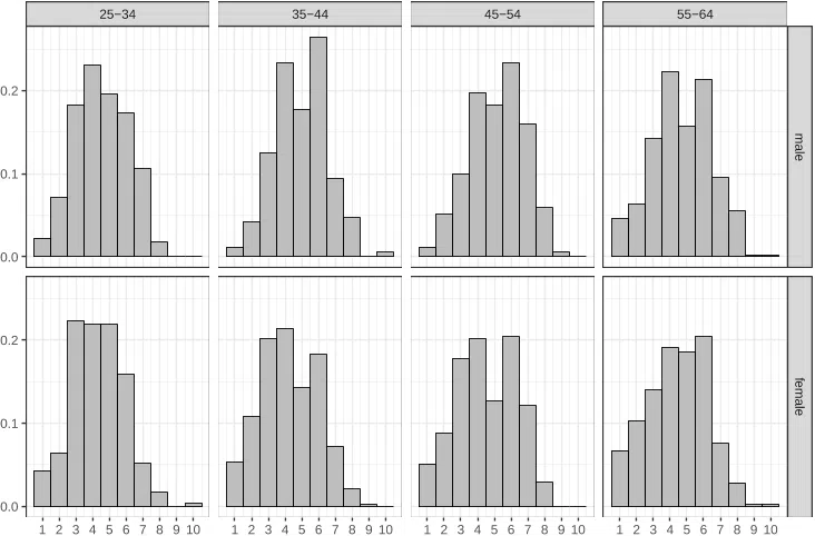
, and Figure 2 shows the distribution of relative evaluation
of income, which ranges from 1 (lowest) to 10 (highest)
2
. Figure 1 shows the
income distribution is well fitted by a lognormal distribution as theoretically
expected (Hamada, 2003, 2004). As for theoretical expectation of the distribu-
tion of income evaluation, if people perceive their income levels correctly, the
distribution is expected to be uniform as will be explained in the next section.
However, Figure 2 shows concentration slightly below the middle point and is
far from a uniform distribution.
[Figure 1 about here.]
[Figure 2 about here.]
These findings lead us to the puzzle of this article which is why the distribu-
tion of the relative evaluation of income level is centralized. The centralization
of the distribution of class identification, which is a multidimensional evaluation
of status, is well known. Several mathematical models have been proposed to
explain this phenomenon (Fararo and Kosaka, 2003; Ishida, 2018). However, to
the best of our knowledge, there are no studies on the mechanism of centraliza-
tion in unidimensional income evaluation. To solve this puzzle, in the following
sections, we introduce a model that assumes that comparisons are made on a
subjective reference distribution of income that is shared among members of a
group rather than the objective income distribution per se.
We first introduce a general model of income evaluation and derive some im-
plications of the model. We then introduce a model imposing the assumption of
1
The unit of income is the Japanese yen. We treated 344 cases with no individual income
and three cases with 100 million yen as missing.
2
The question in the questionnaire was as follows: Thinking about present-day Japanese
society, how would you rate your own level of income below on a scale of 1 (the highest level)
to 10 (the lowest level)?
2

lognormal distribution as the theoretical distribution of income. Next, we con-
duct an empirical data analysis of Japanese survey data by employing Bayesian
statistical modeling, based on the lognormal distribution model. Finally, we
present the conclusions.
2 General Model
In this section, we introduce the model in a general form without specifying the
types of income distribution and subjective reference income distribution. We
then derive some implications.
2.1 Model Assumption
Let Y ∈ {0, ··· , m} be a discrete random variable of response to the m + 1-
scaled income evaluation question, which ranges from 0 (lowest) to m (highest).
Let x ∈ (0, ∞) be the income level of an individual and p be the probability
that x exceeds the income level z, that is, p = Pr(x ≥ z).
We assume that an individual evaluates their relative position of income by
repeatedly comparing themselves with others whom they randomly encounter
on a subjective reference income distribution. It is further assumed that the
subjective reference distribution reflects the biased pattern of an individual’s
daily encounters and/or their expectations about the distribution that are not
based on their experience but on media information or rumors. Here, we make a
baseline assumption that the subjective reference income distribution is identical
and commonly shared among members of a social category, presupposing that
their social experiences and perceptions are almost similar. In addition, when
evaluating their income, the individual is assumed to respond according to the
number of times they have outperformed others in the last m comparisons.
The general model can be composed as
Y ∼ Binomial(m, p), (1)
p = F
s
(x), (2)
x ∼ f
o
(x), (3)
where F
s
is the cumulative distribution function (CDF in short) of the subjective
reference income distribution and f
o
is the probability density function (PDF
in short) of the objective income distribution.
We are ultimately interested in the distribution of Y . However, if m is a
constant, the distribution of Y depends only on the parameter p of the binomial
distribution, so we are essentially interested in the distribution of p. Then, the
PDF of p, denoted as φ(p), is
φ(p) = f
o
(x)
dx
dp
= f
o
(x)
1
{F
s
(x)}
′
=
f
o
(x)
f
s
(x)
.
From equation (2), x can be expressed as the inverse CDF of the subjective
reference distribution, i.e. x = F
−1
s
(p). Finally, we obtain the full form of the
3

PDF of p as
φ(p) =
f
o
(F
−1
s
(p))
f
s
(F
−1
s
(p))
. (4)
By definition, we can confirm the following properties of φ(p), which indicate
that φ(p) is surely a PDF:
φ(p) = f
o
(x)
dx
dp
≥ 0,
Z
1
0
φ(p)dp =
Z
1
0
f
o
(x)
dx
dp
dp
=
Z
∞
−∞
f
o
(x)dx = 1.
2.2 Model Derivations
Henceforth, we assume that f
o
, f
s
is a unimodal and second-order differentiable
PDF. Furthermore, we assume F
s
, which is the CDF of f
s
, is a strictly increasing
function, and F
−1
s
, which is the inverse CDF of f
s
, is also a strictly increasing
and differentiable function.
First, we assume, as a special case, that the subjective reference income
distribution is equal to the objective income distribution, because there is no
encounter bias. That is, f
o
= f
s
. Then, we obtain φ(p) = 1, which means
p is uniformly distributed from 0 to 1. That is, p ∼ Uniform(0, 1). This is an
ideal situation of income evaluation, assumed by the relative income hypothesis,
where people perceive the objective income distribution correctly and evaluate
their income with respect to the exact relative position in the objective income
distribution.
Now, we move on to more general situations where there is a difference
between the objective income distribution and subjective reference income dis-
tribution, which is biased from the objective distribution. That is, f
o
= f
s
.
Differentiating φ(p), which is expressed as equation (4), we obtain the deriva-
tive of φ(p) as
φ
′
(p) =
f
′
o
(x)f
s
(x) − f
o
(x)f
′
s
(x)
f
s
(x)
2
F
−1
s
(p)
′
. (5)
Because f
s
(x) > 0, {F
−1
s
(p)}
′
> 0 on their support from the assumption, the
sign condition of φ
′
(p) solely depends on the relation between the magnitudes
of f
′
o
(x)/f
o
(x) and f
′
s
(x)/f
s
(x) which are the growth rates of PDF of objective
income distribution and subjective income distribution, respectively, that is:
φ
′
(p) ⋛ 0 ⇐⇒
f
′
o
(x)
f
o
(x)
⋛
f
′
s
(x)
f
s
(x)
. (6)
Hence, if there is a point x
∗
that makes the growth rates of both f
o
and f
s
equal,
then the point p
∗
= F
s
(x
∗
) is a lo cal maximum, or minimum, point of φ(p).
For a simple example, if f
′
o
(x
∗
) = f
′
s
(x
∗
) = 0 which indicates both distributions
have the same mode, then the point p
∗
= F
s
(x
∗
) yields φ
′
(p
∗
) = 0.
4

We assume that there is a single point p
∗
such as φ
′
(p
∗
) = 0. The second
derivative at p oint p
∗
is
φ
′′
(p
∗
) =
f
′′
o
(x
∗
)f
s
(x
∗
) − f
o
(x
∗
)f
′′
s
(x
∗
)
f
s
(x
∗
)
2
F
−1
s
(p
∗
)
′
2
. (7)
The sign condition of φ
′′
(p
∗
) depends on the relation between the magnitudes
of f
′′
o
(x)/f
o
(x) and f
′′
s
(x)/f
s
(x), which might be called the growth rate in terms
of second derivative. That is,
φ
′′
(p
∗
) ⋛ 0 ⇐⇒
f
′′
o
(x)
f
o
(x)
⋛
f
′′
s
(x)
f
s
(x)
. (8)
From these derivations, the condition for the appearance of the centraliza-
tion effect in terms of income evaluation can be summarized as follows. There
is a single maximum point that satisfies f
′
o
(x
∗
)/f
o
(x
∗
) = f
′
s
(x
∗
)/f
s
(x
∗
) and
f
′′
o
(x
∗
)/f
o
(x
∗
) < f
′′
s
(x
∗
)/f
s
(x
∗
), and p
∗
= F
s
(x
∗
) is around 0.5.
3 Lognormal Distribution Model
Next, we analyze a more restrictive model, in which both the objective and
subjective reference income distributions are assumed to be lognormally dis-
tributed.
3.1 Model Assumption
Let z ∈ (0, ∞) be an individual’s income, and x = log z be the logged income
ranging from −∞ to ∞. We assume that income z is lognormally distributed as
a common assumption in the field of income distribution studies. Accordingly,
x is normally distributed. That is,
z ∼ Lognormal(µ, σ),
x ∼ Normal(µ, σ).
The PDF of the objective distribution of logged income x, which is a normal
distribution with parameters µ
o
, σ
o
, is denoted by f
o
(x|µ
o
, σ
o
), and that of the
subjective reference distribution, which is a normal distribution with parameters
µ
s
, σ
s
is denoted by f
s
(x|µ
s
, σ
s
). In concrete terms, the PDF can be expressed
as
f
k
(x|µ
k
, σ
k
) =
1
√
2πσ
k
exp
−
(x − µ
k
)
2
2σ
2
k
, (k = o, s). (9)
3.2 Model Derivation
Let us perform some derivation from the model.
First, to determine the condition of a local maximum point of the distribution
p, we specify the growth rate of the objective and subjective reference income
5